Bézier curves are used extensively in computer graphics, often to produce smooth curves. If you have ever used Photoshop you might have stumbled upon that tool called "Anchor" where you can put anchor points and draw some curves with them... These are Bézier curves. Or if you have used vector-based graphic, SVG, these too use Bézier curves. Let's see how it works.
General Definition
Given [begin-latex-inline]n+1[end-latex-inline] points [begin-latex-inline]\{P_0, ..., P_n\}[end-latex-inline] called the control points, the Bézier curve traced by these points is defined as:
Where [begin-latex-inline]P_i=\{x_i, y_i\}[end-latex-inline], and [begin-latex-inline]B_i^n(t)[end-latex-inline] is the Bernstein polynomial:
Notice that Bernstein polynomial looks a lot like the [begin-latex-inline]k^{\text{th}}[end-latex-inline] term in Newton's binomial formula:
For the particular values of [begin-latex-inline]a=1[end-latex-inline] and [begin-latex-inline]b=t-1[end-latex-inline]. It then becomes obvious that:
Therefore, you can interpret [begin-latex-inline]Z(t)[end-latex-inline] as a weighted average of the control points. As [begin-latex-inline]t[end-latex-inline] changes, the weighted average [begin-latex-inline]Z(t)[end-latex-inline] smoothly moves from the first control point to the last control point. Indeed:
That is because:
Similarly:
Quadratic Bézier Curve
The quadratic Bézier curve is how we call the Bézier curve with 3 control points, since the degree of [begin-latex-inline]Z(t)[end-latex-inline] will be 2. Let's calculate the Bézier curve given 3 control points and explore some properties we might find! Remember, [begin-latex-inline](1)[end-latex-inline] holds for [begin-latex-inline]n+1[end-latex-inline] points, so in our case [begin-latex-inline]n=2[end-latex-inline].
Now we just have to choose three control points and evaluate the curve on the range [begin-latex-inline][0, 1][end-latex-inline]. We can do this in Python easily.
import numpy as np
import matplotlib.pyplot as plt

P0, P1, P2 = np.array([
	[0, 0],
	[2, 4],
	[5, 3]
])

# define bezier curve
Z = lambda t: (1 - t)**2 * P0 + 2 * t * (1 - t) * P1 + t**2 * P2

# evaluate the curve on [0, 1] sliced in 50 points
points = np.array([Z(t) for t in np.linspace(0, 1, 50)])

# get x and y coordinates of points separately
x, y = points[:,0], points[:,1]

# plot
plt.plot(x, y, 'b-')
plt.plot(*P0, 'r.')
plt.plot(*P1, 'r.')
plt.plot(*P2, 'r.')
plt.show()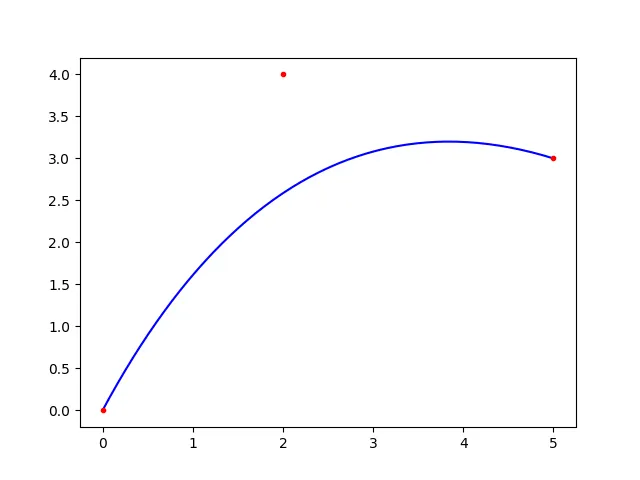
Notice that the curve does indeed start and end at the first and last control points. Because of that, if you fix [begin-latex-inline]P_0[end-latex-inline] and [begin-latex-inline]P_2[end-latex-inline], the [begin-latex-inline]P1[end-latex-inline] entirely determines the shape of the curve. Moving [begin-latex-inline]P1[end-latex-inline] around you might notice something:
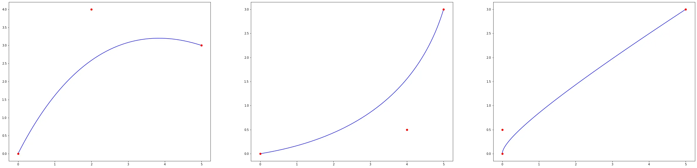
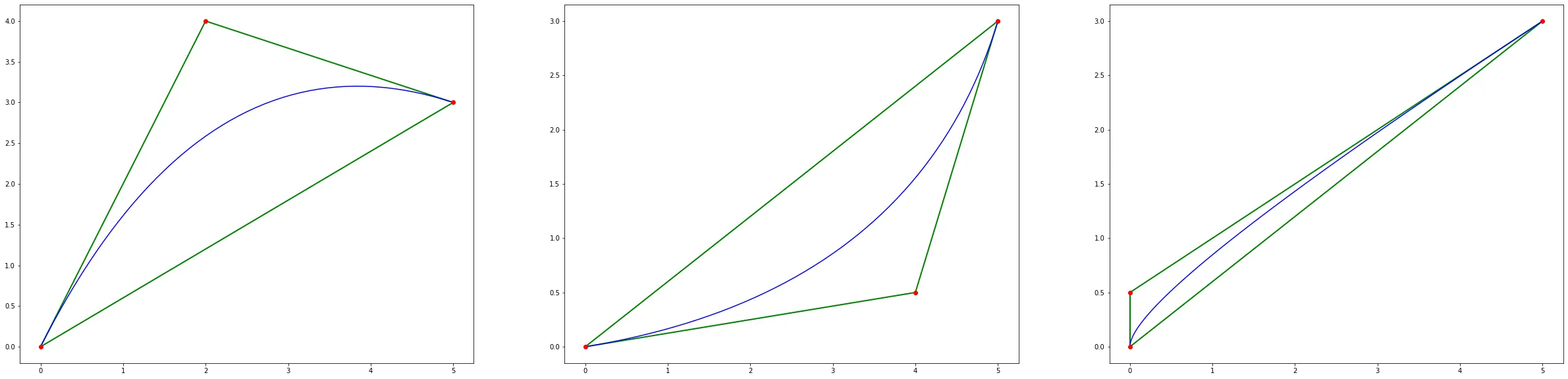
The Bézier curve is always contained in the polygon formed by the control points. This polygon is hence called the control polygon, or Bézier polygon. This property also holds for any number of control points, which makes their manipulation quite intuitive when using a software.
Matrix Representation
We can actually represent the Bézier formula using matrix multiplication, which might be useful in other contexts, for instance for splitting the Bézier curve. If we go back to our example we can rewrite [begin-latex-inline]Z(t)[end-latex-inline] as follows:
All the information of the quadratic Bézier curve is now compacted into one matrix, [begin-latex-inline]M[end-latex-inline]. Notice the [begin-latex-inline]i^{\text{th}}[end-latex-inline] column of [begin-latex-inline]M[end-latex-inline] is just the coefficients of the polynomial [begin-latex-inline]B_i^n[end-latex-inline]. However, if we want to program this, it will be easier to create a matrix row by row, instead of column by column. Luckily, because [begin-latex-inline]{n \choose i} = {n \choose n-i}[end-latex-inline], the [begin-latex-inline]i^{\text{th}}[end-latex-inline] row of the matrix is just the reversed [begin-latex-inline](n-i)^{\text{th}}[end-latex-inline] column.
Therefore, the coefficients of the matrix are nothing but the coefficients of [begin-latex-inline]t[end-latex-inline]:
from math import comb

def get_bezier_matrix(n: int) -> list[list[float]]:
    coef = [[0] * (n + 1) for _ in range(n + 1)]
    for i in range(n + 1):
        for k in range(i + 1):
            coef[i][k] = comb(n, i) * comb(i, k) * (-1)**(i - k)
    return coef
Lastly, this is a general version of the polynomial version:
import numpy as np
import matplotlib.pyplot as plt
from math import comb

def get_bezier_curve(points):
    n = len(points) - 1
    return lambda t: sum(
        comb(n, i) * t**i * (1 - t)**(n - i) * points[i]
        for i in range(n + 1)
    )

def evaluate_bezier(points, total):
    bezier = get_bezier_curve(points)
    new_points = np.array([bezier(t) for t in np.linspace(0, 1, total)])
    return new_points[:,0], new_points[:,1]

points = np.array([
    [0, 0],
    [-1, 3],
    [4, 3],
    [6, 0],
    [7, 2.5]
])

x, y = points[:,0], points[:,1]
bx, by = evaluate_bezier(points, 50)
plt.plot(bx, by, 'b-')
plt.plot(x, y, 'r.')
plt.show()