Finite Difference Method

In this article we will see how to use the finite difference method to solve non-linear differential equations numerically. We will practice on the pendulum equation, taking air resistance into account, and solve it in Python.

We will find the differential equation of the pendulum starting from scratch, and then solve it. Before we start, we need a little background on Polar coordinates.

Polar Coordinates

You already know the famous Cartesian coordinates (x, y, z coordinates), which are probably the most used in everyday life. However, in some cases, describing the position of an object in Cartesian coordinates isn't practical. For instance, when an object is in a circular movement, sine and cosine functions are going to pop all over the place, so it's generally a much better idea to describe that object's position in what we call Polar coordinates.

Polar coordinates are described by two variables, the radius [begin-latex-inline]\rho[end-latex-inline] and the angle [begin-latex-inline]\theta[end-latex-inline]. We attach unit vectors to each variable:

[begin-latex-inline]\vec{e_{\rho}}[end-latex-inline] is a unit vector always pointing in the same direction as vector [begin-latex-inline]\vec{OM}[end-latex-inline].
[begin-latex-inline]\vec{e_{\theta}}[end-latex-inline] is a unit vector perpendicular to [begin-latex-inline]\vec{e_{\rho}}[end-latex-inline].

Our goal now is to express the position, velocity, and acceleration of an object in Polar coordinates. For this we need to express the relationship between the Polar unit vectors and the Cartesian unit vectors.

Cartesian to Polar:

[begin-latex]\begin{align*} &\vec{e_{\rho}} = \cos(\theta) \vec{e_x} + \sin(\theta) \vec{e_y} \\ &\vec{e_{\theta}} = -\sin(\theta) \vec{e_x} + \cos(\theta) \vec{e_y} \end{align*}[end-latex]

Polar to Cartesian:

[begin-latex]\begin{align*} &\vec{e_x} = \cos(\theta) \vec{e_{\rho}} - \sin(\theta) \vec{e_{\theta}} \\ &\vec{e_y} = \sin(\theta) \vec{e_{\rho}} + \cos(\theta) \vec{e_{\theta}} \end{align*}[end-latex]

Good! Now let's express position, velocity, and acceleration in Polar coordinates.

Position

This one is simple, it's the whole point of using Polar coordinates!

[begin-latex]\overrightarrow{OM} = \rho \vec{e_{\rho}}[end-latex]

Velocity

We simply differentiate the position with respect to time. We will assume [begin-latex-inline]\rho[end-latex-inline] is a constant, and only [begin-latex-inline]\theta[end-latex-inline] varies over time.

[begin-latex]\begin{align*} \frac{d\overrightarrow{OM}}{dt} &= \rho \frac{d\vec{e_{\rho}}}{dt} \\ &= \rho \frac{d\vec{e_{\rho}}}{d\theta} \frac{d\theta}{dt} \\ &= \rho (-\sin(\theta) \vec{e_x} + \cos(\theta) \vec{e_y}) \dot{\theta} \\ &= \rho \dot{\theta} \vec{e_{\theta}} \end{align*}[end-latex]

Acceleration

We differentiate the velocity with respect to time.

[begin-latex]\begin{align*} \frac{d^2\overrightarrow{OM}}{dt^2} &= \rho \frac{d\dot{\theta} \vec{e_{\theta}}}{dt} \\ &= \rho \left( \frac{d\dot{\theta}}{dt} \vec{e_{\theta}} + \dot{\theta} \frac{d\vec{e_{\theta}}}{dt} \right) \\ &= \rho \left( \ddot{\theta} \vec{e_{\theta}} + \dot{\theta} \frac{d\vec{e_{\theta}}}{d\theta} \frac{d\theta}{dt} \right) \\ &= \rho \left( \ddot{\theta} \vec{e_{\theta}} - \dot{\theta}^2 \vec{e_{\rho}} \right) \\ &= -\rho \dot{\theta}^2 \vec{e_{\rho}} + \rho \ddot{\theta} \vec{e_{\theta}} \end{align*}[end-latex]

Done! We can now work on our problem: the pendulum.

Pendulum Equation

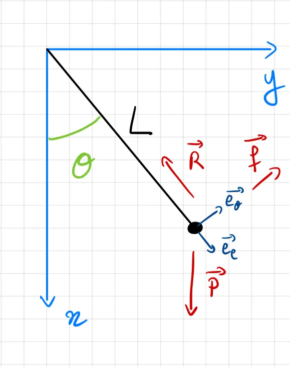
To find the equation that angle [begin-latex-inline]\theta[end-latex-inline] satisfies, we will use Newton's second law of motion, or as we call it in French, the fundamental principle of dynamic.

[begin-latex]\sum{\overrightarrow{F_{\rightarrow \text{system}}}} = m \vec{a}[end-latex]

The sum of all the forces applied to a system is equal to its mass times its acceleration. Let's enumerate all the forces applied to the pendulum and express them in Polar coordinates.

Weight

The weight of the object due to gravity is one of the forces applied to the object. Its formula is well known, mass times gravity, and will be expressed in our coordinate system as:

[begin-latex]\begin{align*} \vec{P} &= mg\vec{e_x} \\ &= mg \cos(\theta) \vec{e_{\rho}} - mg \sin(\theta) \vec{e_{\theta}} \end{align*}[end-latex]

Where [begin-latex-inline]m[end-latex-inline] (kg) is the mass of the object, and [begin-latex-inline]g[end-latex-inline] (m/s²) is value of the acceleration of gravity — which is about 9.81 on Earth.

Rope Tension

The rope exerts a tension pulling the pendulum in the direction of the rope's fixed end.

[begin-latex]\vec{R} = -R \vec{e_{\rho}}[end-latex]

Where [begin-latex-inline]R[end-latex-inline] (N) is the rope tension in Newtons.

Air Resistance

Lastly, the air exerts a friction on the pendulum as it swings, which will make it stop oscillating at some point. Small air resistance is usually modeled as a force opposite to the velocity vector and proportional to the norm of the velocity vector.

[begin-latex]\begin{align*} \vec{f} &= -k \vec{v} \\ &= -kL \dot{\theta} \vec{e_{\theta}} \end{align*}[end-latex]

Where [begin-latex-inline]k[end-latex-inline] (kg/s) is the friction coefficient that is specific to the object in movement, and [begin-latex-inline]L[end-latex-inline] (m) is the length of the pendulum rope.

Note: If something is rotating at angular speed [begin-latex-inline]\omega[end-latex-inline] (rad/s) around an axis at a distance [begin-latex-inline]r[end-latex-inline] (m), then the magnitude of the object's velocity is [begin-latex-inline]r\omega[end-latex-inline] (m/s). For example, the speed of the tip of a fan's blade, or a pendulum (which is why we multiply by [begin-latex-inline]L[end-latex-inline]).

Newton's second law of motion

We can now apply Newton's second law of motion:

[begin-latex]\begin{align*} \vec{P} + \vec{R} + \vec{f} &= m \vec{a} \\ \iff mg \cos(\theta) \vec{e_{\rho}} - mg \sin(\theta) \vec{e_{\theta}} -R \vec{e_{\rho}} -kL \dot{\theta} \vec{e_{\theta}} &= -mL\dot{\theta}^2 \vec{e_{\rho}} + mL\ddot{\theta} \vec{e_{\theta}} \end{align*}[end-latex]

Then project the result on both axes independently:

[begin-latex]\begin{align} mg \cos(\theta) - R = -mL\dot{\theta}^2 \\ - mg \sin(\theta) -kL \dot{\theta} = mL\ddot{\theta} \end{align}[end-latex]

Reordering the terms of [begin-latex-inline](2)[end-latex-inline], we get:

[begin-latex]\ddot{\theta} + \frac{k}{m} \dot{\theta} + \frac{g}{L} \sin(\theta) = 0[end-latex]

Solving this second order non-linear differential equation is complicated. This is where the Finite Difference Method comes very handy. It will boil down to two lines of Python! Let's see how.

Finite Difference Method

The method consists of approximating derivatives numerically using a rate of change with a very small step size.

[begin-latex]f'(x) = \lim_{h \to 0} \frac{f(x+h) - f(x)}{h}[end-latex]

That is the very definition of what a derivative is. Numerically, if we knew [begin-latex-inline]f[end-latex-inline], we could take a small number [begin-latex-inline]h[end-latex-inline] — e.g. 0.0001 — and compute the above formula for a given [begin-latex-inline]x[end-latex-inline], which would give us an approximation of [begin-latex-inline]f'(x)[end-latex-inline].

The finite difference method simply uses that fact to transform differential equations into ordinary equations.

In our case, we start by expressing [begin-latex-inline]\ddot{\theta}[end-latex-inline] with respect to [begin-latex-inline]\dot{\theta}[end-latex-inline] using the rate of change.

[begin-latex]\ddot{\theta}(t) = \frac{\dot{\theta}(t+dt) - \dot{\theta}(t)}{dt}[end-latex]

I removed the limit, and wrote [begin-latex-inline]dt[end-latex-inline] to signal this is an infinitesimal value — in practice, just a very small number. We will now plug this equation into the pendulum equation [begin-latex-inline](2)[end-latex-inline].

[begin-latex]\begin{align*} &\ddot{\theta}(t) + \frac{k}{m} \dot{\theta}(t) + \frac{g}{L} \sin(\theta(t)) = 0 \\ \iff & \frac{\dot{\theta}(t+dt) - \dot{\theta}(t)}{dt} + \frac{k}{m} \dot{\theta}(t) + \frac{g}{L} \sin(\theta(t)) = 0 \\ \iff & \dot{\theta}(t+dt) - \dot{\theta}(t) + dt \frac{k}{m} \dot{\theta}(t) + dt \frac{g}{L} \sin(\theta(t)) = 0 \\ \iff & \dot{\theta}(t+dt) = \dot{\theta}(t) - dt \frac{k}{m} \dot{\theta}(t) - dt \frac{g}{L} \sin(\theta(t)) \end{align*}[end-latex]

Okay! We managed to express the angular velocity at time [begin-latex-inline]t+dt[end-latex-inline] with respect to the angle and angular velocity at time [begin-latex-inline]t[end-latex-inline]. In other words, if for instance [begin-latex-inline]dt=0.001[end-latex-inline] and if you know [begin-latex-inline]\theta(0)[end-latex-inline] and [begin-latex-inline]\dot{\theta}(0)[end-latex-inline] (which are the initial conditions of the system), then you can compute [begin-latex-inline]\dot{\theta}(0.001)[end-latex-inline]! If we could also compute [begin-latex-inline]\theta(0.001)[end-latex-inline] then the recursion is complete and we can compute [begin-latex-inline]\{\theta(t), \dot{\theta}(t)\}[end-latex-inline] for any [begin-latex-inline]t[end-latex-inline] starting with known initial conditions.

Fortunately, there is a way to compute [begin-latex-inline]\theta(t+dt)[end-latex-inline]:

[begin-latex]\begin{align*} &\dot{\theta}(t) = \frac{\theta(t+dt) - \theta(t)}{dt} \\ \iff & \theta(t+dt) = dt \dot{\theta}(t) + \theta(t) \end{align*}[end-latex]

This is again the definition of the derivative, applied to [begin-latex-inline]\dot{\theta}(t)[end-latex-inline]! With that equation in hand we can also compute the angle at time [begin-latex-inline]t+dt[end-latex-inline] given the angle and the angular velocity at time [begin-latex-inline]t[end-latex-inline].

Using these two equations we can now compute the angle [begin-latex-inline]\theta[end-latex-inline] at any time step!

[begin-latex]\left\{ \begin{array}{ll} \dot{\theta}(t+dt) = \dot{\theta}(t) - dt \frac{k}{m} \dot{\theta}(t) - dt \frac{g}{L} \sin(\theta(t)) \\ \theta(t+dt) = dt \dot{\theta}(t) + \theta(t) \end{array} \right.[end-latex]

Given [begin-latex-inline]\{\theta(0), \dot{\theta}(0)\}[end-latex-inline] you can compute [begin-latex-inline]\{\theta(dt), \dot{\theta}(dt)\}[end-latex-inline]. Given [begin-latex-inline]\{\theta(dt), \dot{\theta}(dt)\}[end-latex-inline] you can compute [begin-latex-inline]\{\theta(2dt), \dot{\theta}(2dt)\}[end-latex-inline], and so on.

Python Simulation

import numpy as np
import matplotlib.pyplot as plt

N = 100         # in how many sub pieces we should break a 1 second interval
T = 15          # total duration of the simulation in seconds
dt = 1 / N      # dt
g = 9.81        # acceleration of gravity
L = 1           # pendulum rope length
k = 0.8         # air resistance coefficient
m = 1           # mass of the pendulum

theta = [np.pi / 2]     # initial angle
theta_dot = [0]         # initial angular velocity
t = [0]                 # initial time

for i in range(N * T):
    theta_dot.append(theta_dot[-1] - theta_dot[-1] * dt * k / m - np.sin(theta[-1]) * dt * g / L)
    theta.append(theta_dot[-1] * dt + theta[-1])
    t.append((i + 1) * dt)

plt.plot(t, theta, label='theta')
plt.plot(t, theta_dot, label='theta dot')
plt.legend()
plt.show()

We iteratively compute [begin-latex-inline]\theta(t)[end-latex-inline] and [begin-latex-inline]\dot{\theta}(t)[end-latex-inline] using the formulas we found, and put the results in two separate lists. Running the code produces the following plot.

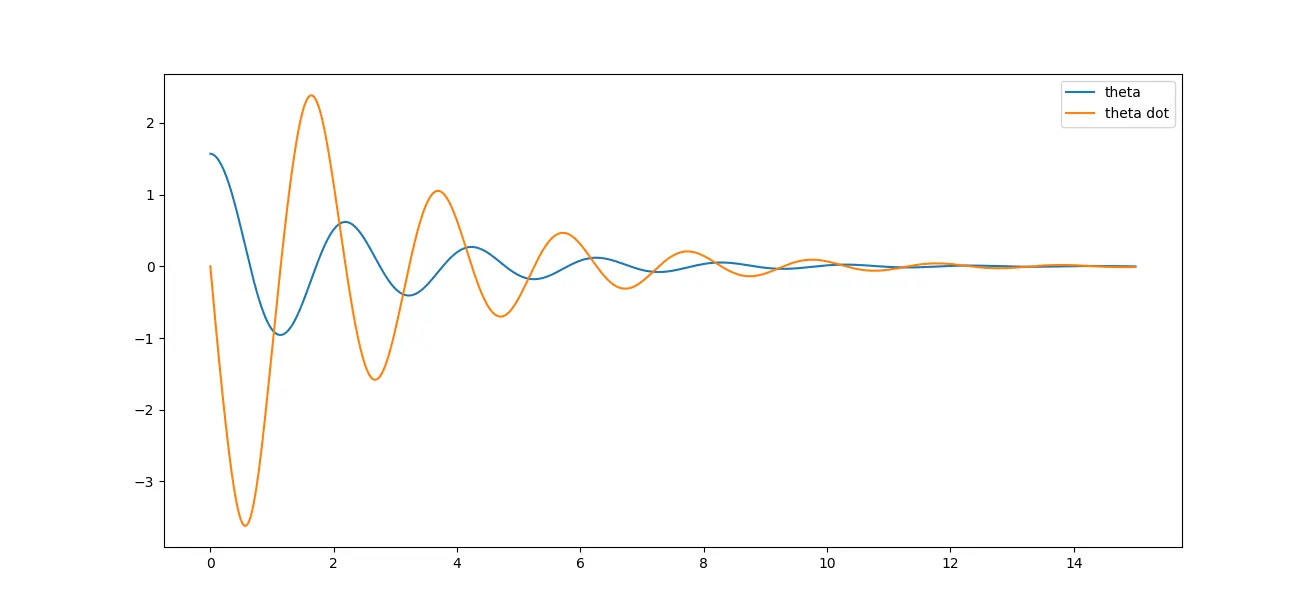
Two happy observations:

The angular velocity seems to reach extremums when the angle is zero, which makes sense since this is where the pendulum has accumulated all its inertia and is about to slow down because it's going up.
The angular velocity seems to reach zero when the angle reaches an extremum, which makes sense since this is when the pendulum is slowing down and is about to go in the other direction.

Playing with the code a little, you might want to set the initial velocity to [begin-latex-inline]2\pi[end-latex-inline] for instance.

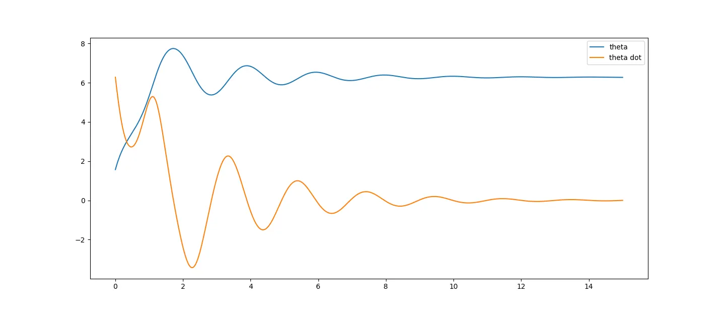
Notice how the angle keeps increasing before going down. What happened is that the initial velocity was high enough to make the pendulum make a full spin before entering the oscillation!

You can try to increase [begin-latex-inline]dt[end-latex-inline] and see how this affects the simulation. We would expect a smaller [begin-latex-inline]dt[end-latex-inline] to give more accurate results (since that controls the approximation of the derivative). Let's see what happens for N=3,2,1.

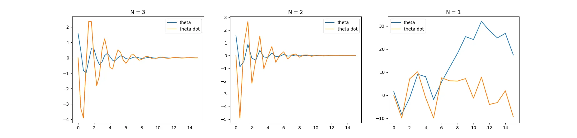
I was actually surprised to see that for only 3 points per second (and even 2), we still manage to get the general shape of the solution. N=1 is another story...