Neural Network From Scratch — Part 2

In part 1 we developed a fully functional neural network library that supports any type of layer, loss function, and optimization method. We then trained a small model to mimic the XOR function.

I can understand how this ending may not be very satisfying given the efforts made to build the library. Thus, in part 2, we extend that library with 2 additional components: Softmax layer, and Cross-Entropy loss, and train a neural network to recognize hand-written digits.

You can find the entire code of the article on my GitHub:

MNIST

The MNIST dataset contains images of hand-written digits from 0 to 9. More precisely, it has 60k training images and 10k test images. Each image is 28x28 pixels, greyscale (0-255). I provide a helper function download_mnist() in the GitHub repository to load the dataset.

>>> x_train, y_train, x_test, y_test = download_mnist()
>>> x_train.shape
(60000, 28, 28)
>>> y_train.shape
(60000,)
>>> x_test.shape
(10000, 28, 28)
>>> y_test.shape
(10000,)

If you plotted the first 15 images of the training set, you'd see this:

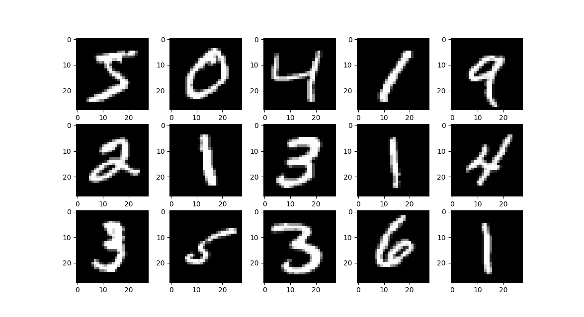
The labels themselves are just the numbers on the images:

>>> print(y_train[:15])
[5 0 4 1 9 2 1 3 1 4 3 5 3 6 1]

The goal is to build a neural network that takes the 28x28 image as input and predicts the label (0-9).

To build this model, we need to add 2 extra components to our library: Softmax and Cross-Entropy. One is an activation function, the other is a loss function.

Softmax

When designing our neural network we have 2 choices for modeling the output:

1. A model that outputs a single number between 0-9.

2. A model that outputs 10 numbers between 0-1, forming a probability distribution over the possible digits. For example, 3 is [begin-latex-inline][0, 0, 0, 1, 0, 0, 0, 0, 0, 0][end-latex-inline].

The first method turns out to work very poorly in practice, and models tend to deal with small numbers a lot better.

So the solution will be to go with 2. However, we want the output to be a probability distribution, i.e. all numbers should sum up to 1, such that we can interpret each number as the probability that the model detected the corresponding digit.

For example, [begin-latex-inline][0, 0.2, 0, 0.7, 0, 0, 0.1, 0, 0, 0][end-latex-inline] is a valid output which reads:

• 20% chance to be 1
• 70% chance to be 3
• 10% chance to be 6

However, there is currently no reason for the neural network to output a set of 10 numbers that sum up to one (in part 1, the last layer was [begin-latex-inline]tanh(x)[end-latex-inline]).

This is what Softmax solves.

Forward Propagation

Because this is not a simple mapping function [begin-latex-inline]\R \to \R[end-latex-inline], we cannot use our Activation module from part 1, this will have to be a separate module. This also means we have to compute [begin-latex-inline]\frac{\partial E}{\partial X}[end-latex-inline].

Backward Propagation

We are given [begin-latex-inline]\frac{\partial E}{\partial Y}[end-latex-inline] and we have to compute [begin-latex-inline]\frac{\partial E}{\partial X}[end-latex-inline] for the previous layer.

[begin-latex-inline]\frac{\partial y_i}{\partial x_k}[end-latex-inline] will change depending on whether [begin-latex-inline]i=k[end-latex-inline] or not, because that will make the numerator of [begin-latex-inline]\sigma(x)_i[end-latex-inline] a variable or a constant with respect to [begin-latex-inline]x_k[end-latex-inline].

If [begin-latex-inline]i=k[end-latex-inline]:

If [begin-latex-inline]i \neq k[end-latex-inline]:

We can now substitute those into the vector form:

Where [begin-latex-inline]\odot[end-latex-inline] is the element-wise product and:

Softmax Code

The implementation is straightforward and we can take advantage of NumPy's broadcasting to avoid building [begin-latex-inline]M[end-latex-inline] ourselves.

class Softmax(Module):
    """Softmax activation layer."""

    def forward(self, inputs: np.ndarray) -> np.ndarray:
        self.outputs = np.exp(inputs)
        self.outputs /= np.sum(self.outputs)
        return self.outputs

    def backward(self, output_grad: np.ndarray) -> np.ndarray:
        n = np.size(self.outputs)
        return np.dot(self.outputs * (np.identity(n) - self.outputs.T), output_grad)

We can verify that this does what we want:

>>> import modules
>>> softmax = modules.Softmax()
>>> softmax.forward([1, 5, 3, 6])
array([0.00473036, 0.25826895, 0.0349529 , 0.70204779])

We now have have a way to force the neural network to output a probability distribution by adding this layer at the end of the network. We could theoretically start training the neural network like we did with XOR using MSE, but in practice this won't work well.

Whenever we have classification tasks, i.e. the network outputs a probability distribution over the possible labels, Cross-Entropy is the go-to loss function. To understand why, I invite you to look at a deeper explanation of the concepts of entropy, cross-entropy, and relative entropy:

Cross-Entropy

The cross-entropy loss is a way to measure the difference between two probability distributions. We are exactly in that case, where the network outputs a certain distribution due to Softmax, but we want to compare that against the actual distribution which is our labels.

If [begin-latex-inline]y^*[end-latex-inline] is the true distribution, and [begin-latex-inline]y[end-latex-inline] is the predicted distribution, then the cross-entropy loss is:

For example, if the true label was [begin-latex-inline][0, 0, 1, 0, 0, 0, 0, 0, 0, 0][end-latex-inline] but the network predicted [begin-latex-inline][0.7, 0, 0.2, 0.1, 0, 0, 0, 0, 0, 0][end-latex-inline], then the cross-entropy loss for that sample would be:

If the prediction was perfect, then we'd have [begin-latex-inline]-log(1)=0[end-latex-inline].

To implement the cross-entropy loss we still need to compute the output gradient:

Therefore, [begin-latex-inline]\frac{\partial E}{\partial Y} = -Y^* \oslash Y[end-latex-inline], where [begin-latex-inline]\oslash[end-latex-inline] is element-wise division.

Cross-Entropy Code

class CrossEntropy(Loss):
    """Cross entropy loss."""

    def loss(self, y_true: np.ndarray, y_pred: np.ndarray) -> float:
        return -np.sum(y_true * np.log(y_pred))

    def loss_prime(self, y_true: np.ndarray, y_pred: np.ndarray) -> np.ndarray:
        return -y_true / y_pred

We are now ready to train on MNIST!

MNIST Solver

Because we have inputs of shape [begin-latex-inline]28 \times 28[end-latex-inline], and we currently only support column vectors, we will flatten our images to vectors of size [begin-latex-inline]28 \times 28=784[end-latex-inline]. It's also a good practice to normalize the inputs; since pixel values are in [begin-latex-inline][0, 255][end-latex-inline], we just divide by [begin-latex-inline]255[end-latex-inline].

def one_hot_encoding(y: np.ndarray, num_classes: int = None) -> np.ndarray:
    y = np.array(y, dtype='int').ravel()
    num_classes = num_classes or np.max(y) + 1
    n = y.shape[0]
    categorical = np.zeros((n, num_classes), dtype='float32')
    categorical[np.arange(n), y] = 1
    return categorical


def preprocess_input(images: np.ndarray, labels: np.ndarray) -> tuple[np.ndarray, np.ndarray]:
    # reshape to one column and normalize
    images = images.astype('float32').reshape(-1, 784, 1) / 255
    # one-hot encoding for labels
    labels = one_hot_encoding(labels).reshape(-1, 10, 1)
    return images, labels


x_train, y_train, x_test, y_test = mnist_loader.download_mnist()
x_train, y_train = preprocess_input(x_train, y_train)
x_test, y_test = preprocess_input(x_test, y_test)

model = modules.Sequential([
    modules.Linear(784, 100),
    modules.Tanh(),
    modules.Linear(100, 50),
    modules.Tanh(),
    modules.Linear(50, 10),
    modules.Softmax()
])

trainer.train(
    model,
    x_train[:3000],
    y_train[:3000],
    losses.CrossEntropy(),
    optimizers.SGD(model, learning_rate=0.001),
    epochs=30,
)

# Compute accuracy over the test set
score = 0
for x, y in zip(x_test, y_test):
    true = np.argmax(y)
    pred = np.argmax(model.forward(x))
    if true == pred:
        score += 1

print(f"Score: {100 * score / len(x_test):.2f}%")

Notice that we're training on the first 3k examples and not the full 60k which can take some time with our current implementation.

1/30 error=3.10702
2/30 error=1.33642
3/30 error=0.88651
...
29/30 error=0.04302
30/30 error=0.04136
Score: 78.24%

This is working!