Q-Learning

Q-Learning is a type of Reinforcement Learning, which is a type of Machine Learning. Reinforcement learning has been used lately to teach AIs to play games (Google DeepMind Atari, etc). Our goal is to understand a simple version of reinforcement learning called Q-Learning, and write a program that will learn to play a simple game.

Preamble

Look at the following code:

class Node:
    def __init__(self, value: int, children: list['Node']):
        self.value = value
        self.children = children


def max_sum(tree: Node) -> int:
    # TODO: find the highest sum for all branches

A Node class is declared to represent a tree structure where each node has a value and some children nodes. A function has to be written: it takes the root of a tree and must return the maximum sum one can get by adding all the values of a given branch of the tree (going from root to leaf without going up). Here's an example where the best path is highlighted in yellow:

digraph MaxPathSumTree { // Graph attributes graph [nodesep=0.3, ranksep=0.5]; edge [fontname="Helvetica"]; // Node definitions A [shape=circle, style=filled, fillcolor=lightgoldenrod1, fontname="Helvetica", penwidth=2, label="10"]; B [shape=circle, style=filled, fillcolor=lightgoldenrod1, fontname="Helvetica", penwidth=2, label="-2"]; C [shape=circle, style=filled, fillcolor=lightblue, fontname="Helvetica", label="10"]; D [shape=circle, style=filled, fillcolor=lightgoldenrod1, fontname="Helvetica", penwidth=2, label="20"]; E [shape=circle, style=filled, fillcolor=lightblue, fontname="Helvetica", label="1"]; F [shape=circle, style=filled, fillcolor=lightblue, fontname="Helvetica", label="-25"]; G [shape=circle, style=filled, fillcolor=lightblue, fontname="Helvetica", label="3"]; H [shape=circle, style=filled, fillcolor=lightblue, fontname="Helvetica", label="4"]; // Edge definitions A -> B; A -> C; B -> D; B -> E; C -> F; F -> G; F -> H; }

Can you complete the function?

This is a typical software engineering interview question. The answer is straightforward:

def max_sum(tree: Node) -> int:
    return tree.value + max([max_sum(child) for child in tree.children], default=0)

This solution recursively finds the best path:

[begin-latex]f(\text{tree}) = \text{value} + \underset{\text{child}}{\max} f(\text{child})[end-latex]

The Bellman equation is basically that, with a bit more theory attached to it:

[begin-latex]Q^*(s, a) = r + \gamma \underset{a'}{\max} Q^*(s', a')[end-latex]

Let's not get ahead of ourselves, and start at the beginning!

Agent & Environment

In Q-Learning, we call the program trying to solve the problem the agent. The agent is going to navigate an environment. The environment is modeled mathematically by a Markov Decision Process, which is a graph where each node is a state the agent may be in (e.g. in a game that would be the position of the user, coins collected, etc.), and where the edges between those nodes are actions the agent can take to transition from one state to another (e.g. right, left, jump, run, etc.). Whenever the agent transitions from one state to another through an action, it receives a reward (a feedback) from the environment, which can be positive or negative. The goal of Q-Learning is to learn a so called Q-function, which tells the agent what action to take in a given state in order to maximize the reward in the long run.

Markov Decision Process

A Markov Decision Process is a mathematical tool to model a system which experiences transition of states with probabilistic rules. This is what we'll use to derive the Bellman equation. Here's an example:

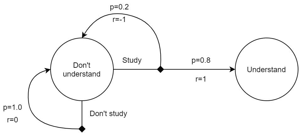
In the graph above, we have:

Two states: Understand and Don't understand
Two actions: Study and Don't study

Here, the probability of understanding given that we currently don't understand and that we study is 80%. The reward for staying in the state of not understanding through the study action is -1.

In Q-learning, this is how we model the environment, and the goal is to maximize the reward we get out of the environment.

Reward

The reward is the feedback from the environment that tells us how good we are doing. It can be the number of coins you grab in a game for example. Our goal is to maximize the total reward.

[begin-latex]R_t = r_{t+1} + r_{t+2} + r_{t+3} + \ldots[end-latex]

We write [begin-latex-inline]R_t[end-latex-inline] to denote the total reward we can get starting at some point [begin-latex-inline]t[end-latex-inline] in time, as the sum of all the subsequent rewards earned at each time step. Defining the reward this way, however, leads to two problems:

The sum could go to infinity, which is a problem since we want to maximize it
We are accounting as much for future rewards as we do for immediate rewards

One way to fix these problems is to use a decreasing factor for future rewards.

[begin-latex]R_t = r_{t+1} + \gamma r_{t+2} + \gamma^2 r_{t+3} + \ldots[end-latex]

Setting [begin-latex-inline]\gamma=1[end-latex-inline] takes us back to the first expression where every reward is equally important. Setting [begin-latex-inline]\gamma=0[end-latex-inline] results in only looking for the immediate reward (greedy policy). Setting [begin-latex-inline]\gamma[end-latex-inline] between [begin-latex-inline]0[end-latex-inline] and [begin-latex-inline]1[end-latex-inline] is a compromise for how much to account for future rewards.

We can rewrite that expression in a recursive manner:

[begin-latex]\begin{align*} R_t &= r_{t+1} + \gamma r_{t+2} + \gamma^2 r_{t+3} + \ldots \\ &= r_{t+1} + \gamma (r_{t+2} + \gamma r_{t+3} + \ldots) \\ &= r_{t+1} + \gamma R_{t+1} \end{align*}[end-latex]

Policy

A policy is a function that tells us what action to take in a certain state. This function is usually denoted [begin-latex-inline]\pi(s,a)[end-latex-inline] and yields the probability of taking action [begin-latex-inline]a[end-latex-inline] in state [begin-latex-inline]s[end-latex-inline]. We want to find the policy that maximizes the reward function.

Since this is a probability distribution, the sum over all the possible actions in a given state must be equal to 1:

[begin-latex]\sum_a \pi(s,a) = 1[end-latex]

Note that this is different from the probabilities on the diagram above, which are the probabilities to end up in some state after taken a given action.

Notations

To derive the Bellman equation, we need to introduce some notations.

[begin-latex]R_{ss'}^a = \mathop{\mathbb{E}} \left[r_{t+1} \quad | \quad s_t=s, a_t=a, s_{t+1}=s'\right][end-latex]

This is the expected immediate reward [begin-latex-inline]r_{t+1}[end-latex-inline] for going from state [begin-latex-inline]s[end-latex-inline] to state [begin-latex-inline]s'[end-latex-inline] through action [begin-latex-inline]a[end-latex-inline].

[begin-latex]P_{ss'}^a = \mathop{\mathbb{P}} \left[s_{t+1}=s' \quad | \quad s_t=s, a_t=a\right][end-latex]

This is the transition probability of going from state [begin-latex-inline]s[end-latex-inline] to state [begin-latex-inline]s'[end-latex-inline] through action [begin-latex-inline]a[end-latex-inline]. In other words, the probability of ending up in state [begin-latex-inline]s'[end-latex-inline] by taking action [begin-latex-inline]a[end-latex-inline] in state [begin-latex-inline]s[end-latex-inline].

Value Functions

We want to take the actions that maximize the reward, but we haven't written any equation that relates both. We can define 2 such functions, that we call value functions.

State Value-Function

We define the "value" of a state as the total expected reward we can get for being in that state and acting according to the policy [begin-latex-inline]\pi[end-latex-inline] from then on. In other words, this is a metric that defines how good it is to be in that state.

[begin-latex]V^\pi(s) = \mathop{\mathbb{E}} \left[R_t \quad | \quad s_t=s\right][end-latex]

State-Action Value-Function

Similarly, we define the "value" of a state-action pair as the total expected reward we can get for being in that state and taking that action, and acting according to the policy [begin-latex-inline]\pi[end-latex-inline] from then on.

[begin-latex]Q^\pi(s,a) = \mathop{\mathbb{E}} \left[R_t \quad | \quad s_t=s, a_t=a\right][end-latex]

Bellman Equation

We can expand the state value-function.

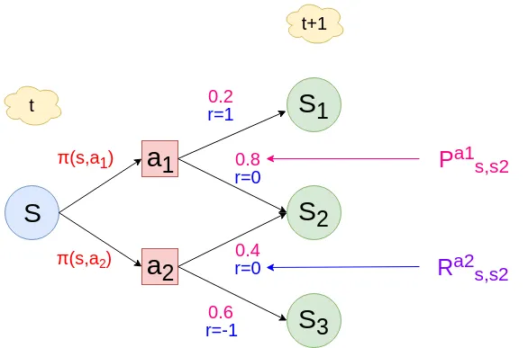
Looking at the following diagram during the calculation can help you understand.

[begin-latex]\begin{align*} V^\pi(s) &= \mathop{\mathbb{E}} \left[R_t \quad | \quad s_t=s\right] \\ &= \sum_a \pi(s,a) Q^{\pi}(s,a) \end{align*}[end-latex]

On the other hand, the state-action value-function is:

[begin-latex]\begin{align*} Q^\pi(s,a) &= \mathop{\mathbb{E}} \left[R_t \quad | \quad s_t=s, a_t=a\right] \\ &= \mathop{\mathbb{E}} \left[r_{t+1} + \gamma R_{t+1} \quad | \quad s_t=s, a_t=a\right] \\ &= \mathop{\mathbb{E}} \left[r_{t+1} \quad | \quad s_t=s, a_t=a\right] + \gamma \mathop{\mathbb{E}} \left[R_{t+1} \quad | \quad s_t=s, a_t=a\right] \\ &= \sum_{s'} P_{ss'}^a R_{ss'}^a + \gamma \sum_{s'} P_{ss'}^a V_{\pi}(s') \end{align*}[end-latex]

We can plug the first equation into the second one to get:

[begin-latex]Q^\pi(s,a) = \sum_{s'} P_{ss'}^a R_{ss'}^a + \gamma \sum_{s'} P_{ss'}^a \sum_{a'} \pi(s',a') Q^{\pi}(s',a')[end-latex]

This, in fact, is a general form of the Bellman equation. But it doesn't really look like the typical "q-function" you may see.

The environment is stochastic: taking an action may lead to different states with different probabilities
The equation describes the value being in state [begin-latex-inline]s[end-latex-inline] and taking action [begin-latex-inline]a[end-latex-inline] given that we act according to the policy [begin-latex-inline]\pi[end-latex-inline] (that we act probabilistically)

If we assume a deterministic environment, then taking an action [begin-latex-inline]a[end-latex-inline] in a state [begin-latex-inline]s[end-latex-inline] always leads to the same state [begin-latex-inline]s'[end-latex-inline]. In that case, [begin-latex-inline]P_{ss'}^a[end-latex-inline] doesn't apply anymore, so we can get rid of it and the sum over possible next states:

[begin-latex]Q^\pi(s,a) = R_{ss'}^a + \gamma \sum_{a'} \pi(s',a') Q^{\pi}(s',a')[end-latex]

And if we now act according to an optimal policy, denoted with a [begin-latex-inline]*[end-latex-inline], then we no longer average over all possible next actions, but instead we pick the action that maximizes the future reward:

[begin-latex]Q^*(s,a) = R_{ss'}^a + \gamma \underset{a'}{\max} Q^*(s',a')[end-latex]

And there we have it!

Python Code

To demonstrate the Bellman Q-Function equation in action, we'll create a small game and train an agent to play that game.

Environment

The environment consists of a 10-by-10 grid. A treasure T is placed at the bottom right corner of the grid. The agent O starts at the top left corner of the grid, and must find the treasure T.

O.........
..........
..........
..........
.........T

The agent can move via the 4 available actions: left, right, up, down.

If the agent takes an action that leads it directly to T then it gets a reward of [begin-latex-inline]1[end-latex-inline], otherwise a reward of [begin-latex-inline]0[end-latex-inline].

import abc


class Env(abc.ABC):
    @abc.abstractmethod
    def actions(self) -> int:
        raise NotImplementedError()

    @abc.abstractmethod
    def states(self) -> int:
        raise NotImplementedError()

    @abc.abstractmethod
    def step(self, action: int) -> tuple[int, int, bool]:
        raise NotImplementedError()

    @abc.abstractmethod
    def reset(self) -> tuple[int, int, bool]:
        raise NotImplementedError()

    @abc.abstractmethod
    def render(self):
        raise NotImplementedError()


class GridEnv(Env):
    def __init__(self, size: int):
        self.x = 0
        self.y = 0
        self.size = size
        self.end_x = size - 1
        self.end_y = size - 1
        self.done = False

    def actions(self) -> int:
        return 4

    def states(self) -> int:
        return self.size ** 2

    def step(self, action: int) -> tuple[int, int, bool]:
        if action == 0:  # left
            self.x = self.x - 1 if self.x > 0 else self.x
        if action == 1:  # right
            self.x = self.x + 1 if self.x < self.size - 1 else self.x
        if action == 2:  # up
            self.y = self.y - 1 if self.y > 0 else self.y
        if action == 3:  # down
            self.y = self.y + 1 if self.y < self.size - 1 else self.y

        done = self.x == self.end_x and self.y == self.end_y
        next_state = self.size * self.y + self.x
        reward = 1 if done else 0
        return next_state, reward, done

    def reset(self) -> tuple[int, int, bool]:
        self.x = 0
        self.y = 0
        self.done = False
        return 0, 0, False

    def render(self):
        for i in range(self.size):
            for j in range(self.size):
                if self.y == i and self.x == j:
                    print("O", end='')
                elif self.end_y == i and self.end_x == j:
                    print("T", end='')
                else:
                    print(".", end='')
            print("")

Q-Learning Algorithm

The idea of the algorithm is to keep a so called q-table, which, over time will approximate the optimal policy [begin-latex-inline]\pi^*(s,a)[end-latex-inline] that maximizes the total reward. Hence, the q-table has a dimension of [begin-latex-inline]\text{states} \times \text{actions}[end-latex-inline]. Initially this table is random.

We start in a state of the environment, and we pick the best action to take according to our q-table. The environment gives us a reward, which we use to update the q-table with the Bellman equation. And we start again.

To allow for exploration, we allow the agent to pick a random action (not the optimal one) with a small probability. This probability decreases over time as the agent becomes better at picking the optimal action.

import os
import env
import time
import random


def train(e: env.Env) -> list[list[float]]:
    qtable = [
        [random.random() for _ in range(e.actions())]
        for _ in range(e.states())
    ]

    # hyperparameters
    epochs = 50
    gamma = 0.1
    epsilon = 0.08
    decay = 0.5

    # training loop
    for i in range(epochs):
        state, reward, done = e.reset()
        steps = 0

        while not done:
            os.system('clear')
            print("epoch #", i+1, "/", epochs)
            e.render()
            time.sleep(0.01)

            # count steps to finish game
            steps += 1

            if random.random() < epsilon:
                # act randomly to allow exploration
                action = random.choice(range(e.actions()))
            else:
                # act greedy and select action with max probability
                action = qtable[state].index(max(qtable[state]))

            # take action
            next_state, reward, done = e.step(action)

            # update qtable value with Bellman equation
            qtable[state][action] = reward + gamma * max(qtable[next_state])

            # update state
            state = next_state

        # The more we learn, the less we take random actions
        epsilon -= decay * epsilon

        print("\nDone in", steps, "steps".format(steps))
        time.sleep(0.8)

    return qtable


grid = env.GridEnv(10)
train(grid)

As the agent trains, it takes shorter and shorter paths to reach the target.