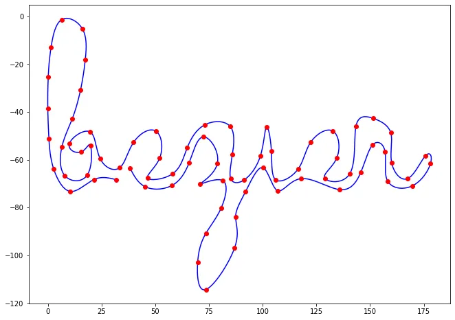
In this article, we'll see how we can use cubic Bézier curves to create a smooth line that goes through a predefined set of points. If you don't know what Bézier curves are, you might want to check this post:
Cubic Bézier Curves
The goal is to fit [begin-latex-inline]n+1[end-latex-inline] given points [begin-latex-inline]{P_0, \ldots, P_n}[end-latex-inline]. In order to fit these points, we'll use one cubic Bézier curve (4 control points) between each consecutive pair of points.
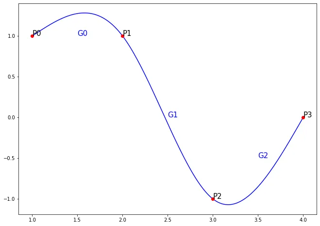
In this figure, [begin-latex-inline]G_0[end-latex-inline], [begin-latex-inline]G_1[end-latex-inline], and [begin-latex-inline]G_2[end-latex-inline] are three different cubic Bézier curves that start and end at [begin-latex-inline](P_0, P_1)[end-latex-inline], [begin-latex-inline](P_1, P_2)[end-latex-inline], and [begin-latex-inline](P_2, P_3)[end-latex-inline] respectively. Since any Bézier curve always starts and ends at the first and last control points, we are left to find 2 control points for each curve.
The general equation of the cubic Bézier curve is the following:
Where [begin-latex-inline]K_i[end-latex-inline] are the 4 control points. In our case, [begin-latex-inline]K_0[end-latex-inline] and [begin-latex-inline]K_3[end-latex-inline] will be two consecutive points that we want to fit (e.g. [begin-latex-inline](P_0, P_1)[end-latex-inline], [begin-latex-inline](P_1, P_2)[end-latex-inline], etc.), and [begin-latex-inline]K_1[end-latex-inline] and [begin-latex-inline]K_2[end-latex-inline] are the 2 remaining control points we have to find. With [begin-latex-inline]t \in [0, 1][end-latex-inline].
Problem Setup
Given that we have [begin-latex-inline]n+1[end-latex-inline] points to fit, we will use a cubic Bézier curve to fit each consecutive pair of points. We denote [begin-latex-inline]\Gamma_i[end-latex-inline] the Bézier curve that fits [begin-latex-inline]P_i[end-latex-inline] to [begin-latex-inline]P_{i+1}[end-latex-inline]:
Where [begin-latex-inline]A_i[end-latex-inline] and [begin-latex-inline]B_i[end-latex-inline] are left to find. Notice that there are [begin-latex-inline]n[end-latex-inline] curves.
If we want the final curve to be smooth, we need to ensure that the transition between [begin-latex-inline]\Gamma_i[end-latex-inline] and [begin-latex-inline]\Gamma_{i+1}[end-latex-inline] is smooth around [begin-latex-inline]P_{i+1}[end-latex-inline]. In other words, that the curvature of [begin-latex-inline]\Gamma_i[end-latex-inline] matches the curvature of [begin-latex-inline]\Gamma_{i+1}[end-latex-inline] around [begin-latex-inline]P_{i+1}[end-latex-inline]. Mathematically, this means respecting the following conditions:
We need to find all [begin-latex-inline]A_i[end-latex-inline] and [begin-latex-inline]B_i[end-latex-inline]. Since we have one pair of them in each Bézier curve, and since we have [begin-latex-inline]n[end-latex-inline] curves, we need to find [begin-latex-inline]2n[end-latex-inline] variables. However, here we have [begin-latex-inline]2(n-1)[end-latex-inline] equations. We are missing 2 equations to solve the system. Therefore, we impose the following (arbitrary) boundary conditions:
Write The System
Before solving the system, we need to calculate the first and second derivatives of [begin-latex-inline]\Gamma_i[end-latex-inline] and write the system down.
Injecting Equations
The boundary condition for the first derivative becomes:
The boundary condition for the second derivative becomes:
The first arbitrary boundary condition becomes:
The second arbitrary boundary condition becomes:
Solve The System
To sum up, we have the following [begin-latex-inline]2n[end-latex-inline] equations where we need to find [begin-latex-inline]A_i[end-latex-inline] and [begin-latex-inline]B_i[end-latex-inline].
To solve the system, we'll eliminate all the [begin-latex-inline]B_i[end-latex-inline] by injecting [begin-latex-inline](1)[end-latex-inline] into [begin-latex-inline](2), (3), (4)[end-latex-inline]. To start off:
Injecting into [begin-latex-inline](2)[end-latex-inline]:
Injecting into [begin-latex-inline](3)[end-latex-inline]:
Injecting into [begin-latex-inline](4)[end-latex-inline]:
Alright! To sump up, after getting rid of [begin-latex-inline]B_i[end-latex-inline], we now have:
We can write this system as a matrix multiplication and solve it!
As you can see, the first matrix is mostly zeros except for the main 3 diagonals. This kind of matrix is called, reasonably enough, a tridiagonal matrix. Algorithms exist to solve this type of systems efficiently, such as Thomas Algorithm which runs linearly in time.
We don't really care about optimizing here. We'll use the built-in function of Numpy in Python to solve the system.
However, we are still missing the [begin-latex-inline]B_i[end-latex-inline] points. To find those, we use equation [begin-latex-inline](1)[end-latex-inline] which works out all the [begin-latex-inline]B_i[end-latex-inline] up until [begin-latex-inline]B_{n-2}[end-latex-inline] and then equation [begin-latex-inline](4)[end-latex-inline] which gives us the last term, [begin-latex-inline]B_{n-1}[end-latex-inline].
We are done at last! Let's see how we can program this using Python.
Python Code
import numpy as np
import matplotlib.pyplot as plt

# find the A & B points
def get_bezier_coef(points):
    # since the formula assumes n+1 points, then n must be:
    n = len(points) - 1

    # build coefficents matrix
    C = 4 * np.identity(n)
    np.fill_diagonal(C[1:], 1)
    np.fill_diagonal(C[:, 1:], 1)
    C[0, 0] = 2
    C[n - 1, n - 1] = 7
    C[n - 1, n - 2] = 2

    # build points vector
    P = [4 * points[i] + 2 * points[i + 1] for i in range(n)]
    P[0] = points[0] + 2 * points[1]
    P[n - 1] = 8 * points[n - 1] + points[n]

    # solve system, find a & b
    A = np.linalg.solve(C, P)
    B = [0] * n
    for i in range(n - 1):
        B[i] = 2 * points[i + 1] - A[i + 1]
    B[n - 1] = (A[n - 1] + points[n]) / 2

    return A, B

# returns the general cubic Bezier formula given 4 control points
def get_bezier_cubic(a, b, c, d):
    return lambda t: np.power(1 - t, 3) * a + 3 * np.power(1 - t, 2) * t * b + 3 * (1 - t) * np.power(t, 2) * c + np.power(t, 3) * d

# returns one cubic Bezier curve for each consecutive pair of points
def get_bezier_interpolation(points):
    A, B = get_bezier_coef(points)
    return [
        get_bezier_cubic(points[i], A[i], B[i], points[i + 1])
        for i in range(len(points) - 1)
    ]

# evalute each cubic Bezier curve on the range [0, 1] sliced in `total` points
def evaluate_bezier_interpolation(points, total):
    curves = get_bezier_interpolation(points)
    return np.array([fun(t) for fun in curves for t in np.linspace(0, 1, total)])


# generate 5 (or any number that you want) random points that we want to fit (or set them youreself)
points = np.random.rand(5, 2)

# fit the points with Bezier interpolation
# use 50 points between each consecutive points to draw the curve
path = evaluate_bezier_interpolation(points, 50)

# extract x & y coordinates of points
x, y = points[:,0], points[:,1]
px, py = path[:,0], path[:,1]

# plot
plt.figure(figsize=(11, 8))
plt.plot(px, py, 'b-')
plt.plot(x, y, 'ro')
plt.show()
Here's a demo running in the browser. Drag the red dots with the mouse to move them around!