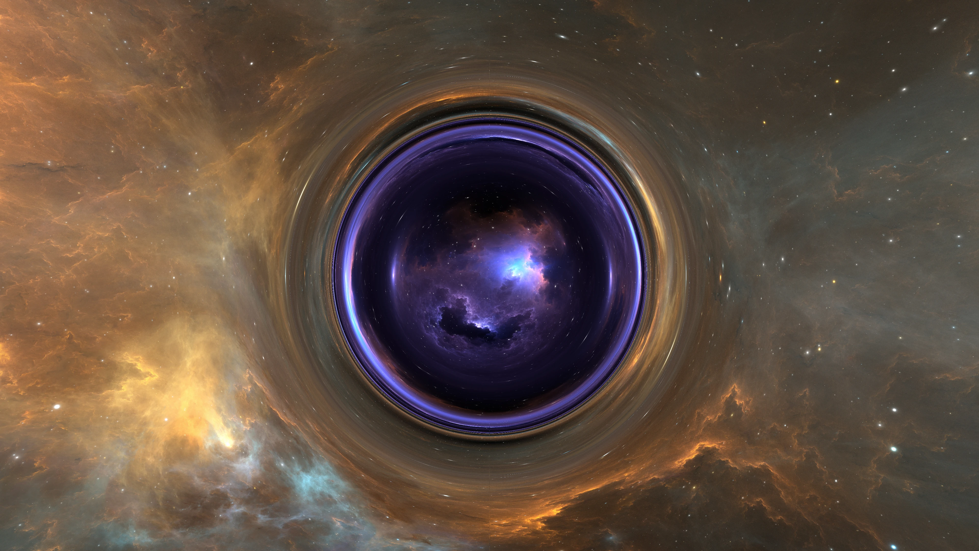
Wormhole — Part 1: Math of General Relativity

Wormholes are theoretical objects (never observed) that are predicted by Einstein's field equations. A wormhole would connect different points of space (and possibly time) and thus act as a shortcut for traveling through the universe. Akin a portal.

Not only wormholes bend the space around them, thus causing light nearby to warp, but light can travel through them which allows us to see the "other side". In this 2-part article, we'll explore the mathematics that describe this fascinating object, and render it with ray tracing. We'll even get to see what it looks like to travel through a wormhole!

Overview

At a high level, to render an image of a wormhole we need:

2 panoramic space images for each side of the wormhole
Set up a virtual scene by defining the position of the camera, the screen, and the wormhole
Shoot rays of light from the camera to each pixel of the screen
Each light ray should follow the geodesic path (straight line in curved space)
If the light ray stays on one side of the wormhole, then we sample a pixel color from one space image, otherwise we sample from the other space image

That's the process in a nutshell. I could give out the equations that describe the path of light and we would embark right-away on the coding journey, but that wouldn't be so fun. Right? In this first part we'll explore fundamental mathematical concepts and derive (as much as we can) the equations that we'll need for our simulation. First stop: the metric tensor.

Metric Tensor

In Euclidean 3D space, a point can be described by Cartesian coordinates [begin-latex-inline](x,y,z)[end-latex-inline]. If we take a small step along each of those axes, we end up at [begin-latex-inline](x+dx,y+dy,z+dz)[end-latex-inline]. The infinitesimal distance between those two points, generally denoted as [begin-latex-inline]dS[end-latex-inline], is:

[begin-latex]dS = \sqrt{dx^2+dy^2+dz^2}[end-latex]

And we could equivalently write:

[begin-latex]dS^2 = dx^2+dy^2+dz^2[end-latex]

It is important to recognize that we used the Pythagorean theorem, which only works in Euclidean space! The formula for the distance between two points changes based on the coordinate system. In general, this [begin-latex-inline]dS^2[end-latex-inline] could be written as the dot-product of the displacement vector with itself:

[begin-latex]\begin{align*} & d\vec{u} = \vec{u}(x+dx, y+dy, z+dz) - \vec{u}(x,y,z) \\ & dS^2 = du^2 = \langle du, du \rangle \end{align*}[end-latex]

Where [begin-latex-inline]\vec{u}[end-latex-inline] is simply the position vector.

Let's do the same operation using polar coordinates. In polar coordinates, we have:

[begin-latex]\begin{align*} x &= r \cos(\theta) \\ y &= r \sin(\theta) \\ \vec{u} &= x \vec{e_x} + y \vec{e_y} \\ &= r \cos(\theta) \vec{e_x} + r \sin(\theta) \vec{e_y} \end{align*}[end-latex]

For a reason that will become clear in a minute, let's also write the basis vectors of the coordinate system, [begin-latex-inline](\vec{e_r}, \vec{e_{\theta}})[end-latex-inline], that are associated with the new variables [begin-latex-inline](r,\theta)[end-latex-inline].

A basis vector for a given coordinate is found by measuring the displacement of the position vector along that coordinate (thus keeping other coordinates fixed). For example, to find the basis vector [begin-latex-inline]\vec{e_r}[end-latex-inline] we fix [begin-latex-inline]\theta[end-latex-inline] to whatever value and only vary [begin-latex-inline]r[end-latex-inline]:

[begin-latex]\begin{align*} \vec{e_r} &= \dfrac{\vec{u}(r+dr, \theta) - \vec{u}(r, \theta)}{dr} \\ & = \dfrac{\partial \vec{u}}{\partial r} \end{align*}[end-latex]

These new vectors span the tangent space at a given point in our new coordinate system. In other words, the basis vectors are pointing in the direction of increasing values of the new coordinates in the immediate vicinity of the point where they're evaluated (i.e. at an infinitesimal scale). Yet in other words, any point in the vicinity of our current position can be described as a linear combination of our basis vectors at our position. These vectors are just the velocity vectors (derivatives of the position vectors).

[begin-latex]\begin{align*} \vec{e_r} &= \dfrac{\partial x}{\partial r} \vec{e_x} + \dfrac{\partial y}{\partial r} \vec{e_y} \\[2ex] &= \cos(\theta) \vec{e_x} + \sin(\theta) \vec{e_y} \\[3ex] \vec{e_{\theta}} &= \dfrac{\partial x}{\partial \theta} \vec{e_x} + \dfrac{\partial y}{\partial \theta} \vec{e_y} \\[2ex] &= -r \sin(\theta) \vec{e_x} + r \cos(\theta) \vec{e_y} \\ \end{align*}[end-latex]

Now, what would be the line differential element [begin-latex-inline]dS^2[end-latex-inline] in polar coordinates? As we said earlier, the Euclidean distance formula does not hold anymore, but we can use vector geometry:

[begin-latex]\begin{align*} d\vec{u}(r,\theta) &= \dfrac{\partial \vec{u}}{\partial r} dr + \dfrac{\partial \vec{u}}{\partial \theta} d\theta \\[3ex] &= \vec{e_r} dr + \vec{e_{\theta}} d\theta \end{align*}[end-latex]

Note that the above is true for any coordinate system. Then we can write:

[begin-latex]\begin{align*} dS^2 &= du^2 \\ &= \langle d\vec{u}, d\vec{u} \rangle \\ &= \langle \vec{e_r} dr + \vec{e_{\theta}} d\theta, \vec{e_r} dr + \vec{e_{\theta}} d\theta \rangle \\ &= \vec{e_r} \cdot \vec{e_r} dr^2 + \vec{e_r} \cdot \vec{e_{\theta}} drd\theta + \vec{e_{\theta}} \cdot \vec{e_r} d\theta dr + \vec{e_{\theta}} \cdot \vec{e_{\theta}} d\theta^2 \\ &= dr^2 + r^2 d\theta^2 \end{align*}[end-latex]

Details:

([begin-latex-inline]\vec{e_x} \cdot \vec{e_x} = 1[end-latex-inline] and [begin-latex-inline]\vec{e_x} \cdot \vec{e_y} = 0[end-latex-inline])

[begin-latex]\begin{align*} \vec{e_r} \cdot \vec{e_r} &= \langle \cos(\theta) \vec{e_x} + \sin(\theta) \vec{e_y}, \cos(\theta) \vec{e_x} + \sin(\theta) \vec{e_y} \rangle \\ &= \cos^2(\theta) \vec{e_x} \cdot \vec{e_x} + \cos(\theta)\sin(\theta) \vec{e_x} \cdot \vec{e_y} + \sin^2(\theta) \vec{e_y} \cdot \vec{e_y} \\ &= \cos^2(\theta) + \sin^2(\theta) \\ &= 1 \end{align*}[end-latex]

[begin-latex]\begin{align*} \vec{e_{\theta}} \cdot \vec{e_{\theta}} &= \langle -r \sin(\theta) \vec{e_x} + r \cos(\theta) \vec{e_y}, -r \sin(\theta) \vec{e_x} + r \cos(\theta) \vec{e_y} \rangle \\ &= r^2 \sin^2(\theta) \vec{e_x} \cdot \vec{e_x} -2 r^2 \cos(\theta) \sin(\theta) \vec{e_x} \cdot \vec{e_y} + r^2 \cos^2(\theta) \vec{e_y} \cdot \vec{e_y} \\ &= r^2 \sin^2(\theta) + r^2 \cos^2(\theta) \\ &= r^2 \end{align*}[end-latex]

[begin-latex]\begin{align*} \vec{e_r} \cdot \vec{e_{\theta}} &= \langle \cos(\theta) \vec{e_x} + \sin(\theta) \vec{e_y}, -r \sin(\theta) \vec{e_x} + r \cos(\theta) \vec{e_y} \rangle \\ &= -r \cos(\theta) \sin(\theta) \vec{e_x} \cdot \vec{e_x} + r \cos^2(\theta) \vec{e_x} \cdot \vec{e_y} - r \sin^2(\theta) \vec{e_y} \cdot \vec{e_x} + r \cos(\theta) \sin(\theta) \vec{e_y} \cdot \vec{e_y} \\ &= 0 \end{align*}[end-latex]

Therefore:

[begin-latex-inline]\|\vec{e_r}\| = 1[end-latex-inline]
[begin-latex-inline]\|\vec{e_{\theta}}\| = r[end-latex-inline]
[begin-latex-inline]\vec{e_r} \perp \vec{e_{\theta}}[end-latex-inline]

If we take a step back, we see that those coefficients of the line element [begin-latex-inline]dS^2[end-latex-inline] are nothing but all pairwise dot products of the basis vectors. We can put those coefficients into a tensor which we call the metric tensor:

[begin-latex]\begin{align*} g_{ij} &= \begin{bmatrix} \vec{e_r} \cdot \vec{e_r} & \vec{e_r} \cdot \vec{e_{\theta}} \\ \vec{e_{\theta}} \cdot \vec{e_r} & \vec{e_{\theta}} \cdot \vec{e_{\theta}} \\ \end{bmatrix} \\[3ex] &= \begin{bmatrix} 1 & 0 \\ 0 & r^2 \\ \end{bmatrix} \end{align*}[end-latex]

The metric tensor describes the entire geometry of the space: how distances and angles are measured within that space. Because the line element contains all the non-zero elements of the metric tensor, we often equivalently represent the metric by the line element directly, e.g.:

[begin-latex]dS^2 = dr^2 + r^2d\theta^2[end-latex]

Interpreting the Metric Tensor

Since the metric tensor contains the dot product of all pairs of basis vectors, it gives us information about distances and angles within that space.

Distances

The diagonal elements of the tensor are just the squares of the basis vector's norms: [begin-latex-inline]\|\vec{e_r}\|^2[end-latex-inline] and [begin-latex-inline]\|\vec{e_{\theta}}\|^2[end-latex-inline]. Therefore, the square root of the diagonal elements tells us how the space is stretched or shrunk along those dimensions.

The polar metric tensor tells us distances along [begin-latex-inline]\vec{e_r}[end-latex-inline] are kept unchanged: one unit of polar coordinate distance along [begin-latex-inline]\vec{e_r}[end-latex-inline] corresponds to one unit of cartesian coordinate distance. While one unit of polar coordinate distance along [begin-latex-inline]\vec{e_{\theta}}[end-latex-inline] scales linearly with [begin-latex-inline]r[end-latex-inline] in cartesian coordinate distance. This makes sense, for a given angle, the further away from the center the longer is the arc travelled: [begin-latex-inline]r\theta[end-latex-inline].

Angles

The off-diagonal elements inform us on how the basis vectors are skewed with respect to each other, or in other words what is the angle between them. Since the dot product of two vectors is nothing but:

[begin-latex]\begin{align*} \vec{a} \cdot \vec{b} &= ub \\ &= va \\ &= ab \cos(\theta) \end{align*}[end-latex]

We can get the actual angle between two pairs of basis vectors from the metric tensor by calculating:

[begin-latex]\theta_{ij} = \arccos \left( \dfrac{g_{ij}}{\sqrt{g_{ii} g_{jj}}} \right)[end-latex]

When the off-diagonal elements of the metric tensor are 0, we can conclude that the basis vectors are orthogonal, because [begin-latex-inline]\vec{a} \cdot \vec{b} = 0 \iff \vec{a} \perp \vec{b}[end-latex-inline]. In comparison to polar coordinates, the metric tensor for the Cartesian coordinate system is:

[begin-latex]g_{ij} = \begin{bmatrix} 1 & 0 & 0 \\ 0 & 1 & 0 \\ 0 & 0 & 1 \end{bmatrix}[end-latex]

Which indicates that:

[begin-latex-inline]\|\vec{e_x}\|=\|\vec{e_y}\|=\|\vec{e_z}\|=1[end-latex-inline]
[begin-latex-inline]\|\vec{e_x}\| \perp \|\vec{e_y}\| \perp \|\vec{e_z}\|[end-latex-inline]

Summary

Given any coordinate system [begin-latex-inline](x^1, x^2, \ldots, x^n)[end-latex-inline], we can define the displacement vector between two nearby points:

[begin-latex]d\vec{X} = dx^i \vec{e_{x_i}}[end-latex]

This way of writing is called the Einstein's summation notation, it's useful for achieving brevity. When an index variable appears twice in a single term and is not otherwise defined, it implies summation of that term over all the values of the index: [begin-latex-inline]d\vec{X} = \sum_{i} dx^i \vec{e_{x_i}}[end-latex-inline]

From there, we can write the infinitesimal line element [begin-latex-inline]dS^2[end-latex-inline] which is the length squared of that displacement:

[begin-latex]\begin{align*} dS^2 &= \langle d\vec{X}, d\vec{X} \rangle \\[2ex] &= \vec{e_{x_i}} \cdot \vec{e_{x_j}} dx^i dx^j \\[2ex] &= g_{ij} dx^i dx^j \end{align*}[end-latex]

This is again using Einstein's summation notation, so a double sum over [begin-latex-inline]i[end-latex-inline] and [begin-latex-inline]j[end-latex-inline] is implied.

The line element is fully determined by the coefficients of each [begin-latex-inline]dx^i dx^j[end-latex-inline] term. Therefore, we can equally define the line element by the metric tensor which contains only those coefficients:

[begin-latex]\begin{align*} g_{ij} &= \begin{bmatrix} \vec{e_{x_1}} \cdot \vec{e_{x_1}} & \vec{e_{x_1}} \cdot \vec{e_{x_2}} & \cdots & \vec{e_{x_1}} \cdot \vec{e_{x_n}} \\ \vec{e_{x_2}} \cdot \vec{e_{x_1}} & \vec{e_{x_2}} \cdot \vec{e_{x_2}} & \cdots & \vec{e_{x_2}} \cdot \vec{e_{x_n}} \\ \vdots & \vdots & \ddots & \vdots \\ \vec{e_{x_n}} \cdot \vec{e_{x_1}} & \vec{e_{x_n}} \cdot \vec{e_{x_2}} & \cdots & \vec{e_{x_n}} \cdot \vec{e_{x_n}} \end{bmatrix} \\ \\ &= \begin{bmatrix} \|\vec{e_{x_1}}\|^2 & \vec{e_{x_1}} \cdot \vec{e_{x_2}} & \cdots & \vec{e_{x_1}} \cdot \vec{e_{x_n}} \\ \vec{e_{x_2}} \cdot \vec{e_{x_1}} & \|\vec{e_{x_2}}\|^2 & \cdots & \vec{e_{x_2}} \cdot \vec{e_{x_n}} \\ \vdots & \vdots & \ddots & \vdots \\ \vec{e_{x_n}} \cdot \vec{e_{x_1}} & \vec{e_{x_n}} \cdot \vec{e_{x_2}} & \cdots & \|\vec{e_{x_n}}\|^2 \end{bmatrix} \end{align*}[end-latex]

Also note that since [begin-latex-inline]\vec{a} \cdot \vec{b} = \vec{b} \cdot \vec{a}[end-latex-inline], the metric tensor is symmetric.

Measure Distances

Given the infinitesimal line element we can measure actual physical distances in space. For example, this is the metric of Euclidean space in spherical coordinates:

[begin-latex]dS^2=dr^2+r^2d\theta^2+r^2\sin^2(\theta)d\phi^2[end-latex]

Where:

[begin-latex-inline]r \in [0, +\infin[[end-latex-inline] is the distance to the origin
[begin-latex-inline]\theta \in [0, \pi][end-latex-inline] is the polar angle (from [begin-latex-inline]+z[end-latex-inline] to [begin-latex-inline]-z[end-latex-inline])
[begin-latex-inline]\phi \in [0, 2\pi][end-latex-inline] is the azimuthal angle (from [begin-latex-inline]x^+[end-latex-inline] to [begin-latex-inline]x^-[end-latex-inline])

This is saying that if we were at [begin-latex-inline](r=5,\theta=\frac{\pi}{2},\phi=0)[end-latex-inline] and took an infinitesimal step of [begin-latex-inline](0.001, 0.002, 0.003)[end-latex-inline] along each of those dimensions, then the total physical distance travelled is:

[begin-latex]\begin{align*} dS &= \sqrt{0.001^2+ 5^2 * 0.002^2 + 5^2\sin^2\left(\frac{\pi}{2}\right) 0.003^2} \\[3ex] &= 0.018 \end{align*}[end-latex]

This, however, is only true as long as we're taking small enough steps [begin-latex-inline](dr,d\theta,d\phi)[end-latex-inline]. To get distances for larger steps, i.e. between arbitrary points, we need to integrate the infinitesimal line element.

In general, to measure the distance between two points that vary in all three coordinates, we would parameterize all three variables, for example with time: [begin-latex-inline]\left(r(t), \theta(t), \phi(t)\right)[end-latex-inline]. So we can write:

[begin-latex]\begin{align*} dr &= \frac{dr}{dt}dt \\[3ex] &= \dot{r} dt \end{align*}[end-latex]

And similarly for [begin-latex-inline]\theta[end-latex-inline] and [begin-latex-inline]\phi[end-latex-inline], then:

[begin-latex]\begin{align*} & dS^2 = \dot{r}^2 dt^2 + r^2 \dot{\theta}^2 dt^2 + r^2 \sin^2(\theta) \dot{\phi}^2 dt^2 \\[3ex] \iff & dS = \sqrt{\dot{r}^2 + r^2 \dot{\theta}^2 + r^2 \sin^2(\theta) \dot{\phi}^2 \\} dt \\[3ex] \iff & S = \int_{t_0}^{t_1} \sqrt{\dot{r}^2 + r^2 \dot{\theta}^2 + r^2 \sin^2(\theta) \dot{\phi}^2 \\} dt \end{align*}[end-latex]

This isn't easy to integrate, but solving it would give the Euclidean arc length of the 3D curve [begin-latex-inline]\left(r(t), \theta(t), \phi(t)\right)[end-latex-inline] from [begin-latex-inline]t_0[end-latex-inline] to [begin-latex-inline]t_1[end-latex-inline].

For example, I can parameterize [begin-latex-inline](r, \theta, \phi)[end-latex-inline] to change linearly from [begin-latex-inline](r_0, \theta_0, \phi_0)[end-latex-inline] to [begin-latex-inline](r_1, \theta_1, \phi_1)[end-latex-inline], and the integral above would give the length of that path:

We can also use the metric to measure distances while varying only a single coordinate (in which case we don't need to parameterize). For example, we might want to fix [begin-latex-inline]r=R[end-latex-inline] and [begin-latex-inline]\theta=\frac{\pi}{2}[end-latex-inline] (equatorial slice) and measure distances along the [begin-latex-inline]\phi[end-latex-inline] axis. If [begin-latex-inline]r[end-latex-inline] and [begin-latex-inline]\theta[end-latex-inline] are constants, then [begin-latex-inline]dr = d\theta = 0[end-latex-inline] and:

[begin-latex]\begin{align*} & dS^2 = R^2 \sin^2\left(\frac{\pi}{2}\right) d\phi^2 \\[3ex] \iff & dS = R d\phi \\[3ex] \iff & S = R \int_{\phi_0}^{\phi_1} d\phi \\[3ex] \iff & S = R (\phi_1 - \phi_0) \end{align*}[end-latex]

We found the formula of the arc length of a circle. For example, measuring the arc length between [begin-latex-inline]\phi_0=0[end-latex-inline] and [begin-latex-inline]\phi_1=2\pi[end-latex-inline] yields the circumference formula [begin-latex-inline]2\pi R[end-latex-inline].

Wormhole Metric

It turns out, there's a particular metric that describes space around a wormhole! The following is the Morris-Thorne metric for a static traversable wormhole:

[begin-latex]dS^2 = -dt^2 + \dfrac{dr^2}{1 - \dfrac{b(r)}{r}} + r^2 d\theta^2 + r^2 \sin^2(\theta) d\phi^2[end-latex]

The Morris-Thorne wormhole metric is described in spherical coordinates, where the wormhole itself is in fact a sphere of radius [begin-latex-inline]r_0[end-latex-inline] at the origin.

Notice the common terms with the Euclidean spherical coordinates:
[begin-latex-inline]dS^2=dr^2+r^2d\theta^2+r^2\sin^2(\theta)d\phi^2[end-latex-inline]

The wormhole metric is written in a 4-variable coordinate system [begin-latex-inline][t,r,\theta,\phi][end-latex-inline], where:

[begin-latex-inline]t \in [-\infin, +\infin[[end-latex-inline]: this is the global time for distant static observers. We'll explain the presence of the minus sign in front of [begin-latex-inline]dt^2[end-latex-inline] later in the article.
[begin-latex-inline]r \in [r_0, +\infin[[end-latex-inline]: this should be interpreted as representing the two-sphere of surface [begin-latex-inline]4\pi r^2[end-latex-inline] and not as the distance to the origin. This is because the coefficient of the [begin-latex-inline]dr^2[end-latex-inline] term is not a constant, therefore distances vary depending on how far we are from the origin of the coordinate system. Notice that the minimum value of [begin-latex-inline]r[end-latex-inline] is [begin-latex-inline]r_0[end-latex-inline], this is the radius of the so-called "throat" of the wormhole. When we travel through the wormhole, [begin-latex-inline]r[end-latex-inline] goes from [begin-latex-inline]+\infin[end-latex-inline] down to [begin-latex-inline]r_0[end-latex-inline] (in one universe) then from [begin-latex-inline]r_0[end-latex-inline] back up to [begin-latex-inline]+\infin[end-latex-inline] (in the other universe). So this variable [begin-latex-inline]r[end-latex-inline] spans 2 spheres (universes).
[begin-latex-inline]\theta \in [0, \pi][end-latex-inline]: the polar angle, i.e. the angle that goes from north to south pole (from [begin-latex-inline]+z[end-latex-inline] to [begin-latex-inline]-z[end-latex-inline])
[begin-latex-inline]\phi \in [0, 2\pi][end-latex-inline]: the azimuthal angle, i.e. the angle that revolves around the sphere (from [begin-latex-inline]x^+[end-latex-inline] to [begin-latex-inline]x^-[end-latex-inline])

So this looks similar to the metric of Euclidean space in spherical coordinates in [begin-latex-inline]\theta[end-latex-inline] and [begin-latex-inline]\phi[end-latex-inline], but not in [begin-latex-inline]r[end-latex-inline]. Notably, there's this factor [begin-latex-inline]\frac{1}{1-\frac{b(r)}{r}}[end-latex-inline] that we haven't yet explained.

[begin-latex-inline]b(r)[end-latex-inline] is the shape function and describes the geometry of the wormhole's throat. First, notice how as long as [begin-latex-inline]b(r) \underset{r \to +\infin}{\sim} o(r)[end-latex-inline] then:

[begin-latex]\underset{r \to +\infin}{\lim} \dfrac{1}{1-\dfrac{b(r)}{r}} = 1[end-latex]

Note: [begin-latex-inline]b(r) \underset{r \to +\infin}{\sim} o(r) \iff \underset{r \to +\infin}{\lim} \dfrac{b(r)}{r} = 0[end-latex-inline]

This means that as we get further away from the origin, the space becomes more and more similar to the metric of Euclidean space in spherical coordinates: the space becomes flat. We say that the space is asymptotically flat.

Similarly, if [begin-latex-inline]b(r)=0[end-latex-inline] then the metric becomes that of flat space as well: there is no wormhole at all.

Physically, one such valid shape function is [begin-latex-inline]b(r)=\dfrac{r_0^2}{r}[end-latex-inline].

As you can see, the [begin-latex-inline]dr^2[end-latex-inline] coefficient goes to [begin-latex-inline]1[end-latex-inline] at infinity, that of the flat Euclidean space. However, this form of the metric is not very convenient because it contains a geometrical singularity at [begin-latex-inline]r=r_0[end-latex-inline]. For our simulation, it will be easier to not deal with the areal radius [begin-latex-inline]r[end-latex-inline] but instead use the actual physical distance to the center of the coordinate system, [begin-latex-inline]l[end-latex-inline]. To get there, we can do a change of variable such that the [begin-latex-inline]dr^2[end-latex-inline] coefficient becomes constant. [begin-latex-inline]l[end-latex-inline] is also called the proper distance and represents the distance travelled along the radial direction.

[begin-latex]\begin{align*} & dl^2 = \frac{dr^2}{1 - \frac{b(r)}{r}} \\[3ex] \iff & dl = \frac{dr}{\sqrt{1 - \frac{b(r)}{r}}} \\[3ex] \iff & l(r) = \int_{r_0}^{r} \frac{dr'}{\sqrt{1 - \frac{b(r')}{r'}}} \end{align*}[end-latex]

By integrating the radial component starting from [begin-latex-inline]r_0[end-latex-inline], we ensure that [begin-latex-inline]l=0[end-latex-inline] at the throat. Then, the metric becomes:

[begin-latex]dS^2 = -dt^2 + dl^2 + r(l)^2 d\theta^2 + r(l)^2 \sin^2(\theta) d\phi^2[end-latex]

Where [begin-latex-inline]r(l)[end-latex-inline] is the reciprocal function of [begin-latex-inline]l(r)[end-latex-inline]. We can compute it for our choice of [begin-latex-inline]b(r)=\dfrac{r_0^2}{r}[end-latex-inline].

[begin-latex]\begin{align*} l(r) &= \int_{r_0}^{r} \frac{dr'}{\sqrt{1 - \frac{b(r')}{r'}}} \\[3ex] &= \int_{r_0}^{r} \frac{dr'}{\sqrt{1 - \frac{r_0^2}{r'^2}}} \\[3ex] &= \int_{r_0}^{r} \frac{r'}{\sqrt{r'^2 - r_0^2}}dr' \\[3ex] &= \left[ \sqrt{r'^2 - r_0^2} \right]_{r_0}^r \\[3ex] &= \sqrt{r^2 - r_0^2} \end{align*}[end-latex]

We can now invert the function to find that [begin-latex-inline]r(l)=\sqrt{l^2+r_0^2}[end-latex-inline]. We can also notice that [begin-latex-inline]r(l)[end-latex-inline] does not have any singularity at [begin-latex-inline]0[end-latex-inline] unlike the areal radius:

Since [begin-latex-inline]r(l)[end-latex-inline] is conveniently symmetric, [begin-latex-inline]r(l)=r(-l)[end-latex-inline], we can extend the range of [begin-latex-inline]l[end-latex-inline] to [begin-latex-inline]]-\infin, +\infin[[end-latex-inline] where [begin-latex-inline]l>0[end-latex-inline] corresponds to one universe, [begin-latex-inline]l<0[end-latex-inline] corresponds to the other, and [begin-latex-inline]l=0[end-latex-inline] at the throat.

In a flat space the radial distance would be simply [begin-latex-inline]\int_{0}^{l}dl'=l[end-latex-inline], which is plotted in red for reference. As expected, here too at infinity, the radial distance in the wormhole space converges towards that of the flat space: [begin-latex-inline]\underset{l \to +\infin}{\lim} \sqrt{l^2+r_0^2} = l[end-latex-inline].

Equatorial Slice Embedding

The wormhole space is curved everywhere near the origin. We can't visualize this properly as it would require a 4D plot. We can however take a single "slice" of the universe, i.e. a plane, and see how space is curved over that surface on a 3D plot. This is what we call a surface embedding. We can visuailze the space distortion at the equator, i.e. [begin-latex-inline]\theta=\frac{\pi}{2}[end-latex-inline], because it makes the calculation easier, but it would be the same everywhere since the space is symmetrical around the origin. With [begin-latex-inline]t=\text{cst}, \theta=\frac{\pi}{2}[end-latex-inline] and therefore [begin-latex-inline]dt=d\theta=0[end-latex-inline], we have:

[begin-latex]dS^2 = dl^2 + r(l)^2 d\phi^2[end-latex]

We end up with a metric spanning the surface area of a cylinder, i.e. [begin-latex-inline]\left(l, \phi\right)[end-latex-inline]. To visualize this surface we need to map it to [begin-latex-inline](x,y,z)[end-latex-inline] coordinates:

[begin-latex]\begin{align*} x &= r(l) \cos(\phi) \\ y &= r(l) \sin(\phi) \\ z &= z(l) \end{align*}[end-latex]

We need to find [begin-latex-inline]z(l)[end-latex-inline] which will describe the shape of the cylinder. We can find it by calculating the line element in the [begin-latex-inline](x,y,z)[end-latex-inline] coordinates then mapping back to [begin-latex-inline]dS^2[end-latex-inline] in the wormhole space.

[begin-latex]\begin{align*} dx &= r'(l) \cos(\phi) dl - r(l) \sin(\phi) d\phi \\ dy &= r'(l) \sin(\phi) dl + r(l) \cos(\phi) d\phi \\ dz &= z'(l) dl \\ \end{align*}[end-latex]

We use the metric in Euclidean space using Cartesian coordinates, which simplifies to:

[begin-latex]\begin{align*} dS^2 &= dx^2 + dy^2 + dz^2 \\ &= (r'(l)^2 + z'(l)^2) dl^2 + r(l)^2 d\phi^2 \end{align*}[end-latex]

By identifying the coefficients with the equatorial slice metric, we find that:

[begin-latex]\begin{align*} & r'(l)^2 + z'(l)^2 = 1 \\ \iff & z'(l) = \sqrt{1 - r'(l)^2} \end{align*}[end-latex]

For our choice of [begin-latex-inline]r(l)=\sqrt{l^2+r_0^2}[end-latex-inline], we have:

[begin-latex]\begin{align*} z'(l) &= \sqrt{1 - r'(l)^2} \\[3ex] &= \sqrt{1 - \frac{l^2}{l^2+r_0^2}} \\[3ex] &= \sqrt{\frac{r_0^2}{l^2+r_0^2}} \\[3ex] &= \frac{1}{\sqrt{\frac{l^2}{r_0^2}+1}} \end{align*}[end-latex]

Finally, we integrate to find that:

[begin-latex]\begin{align*} z(l) &= \int_0^l \frac{dl'}{\sqrt{\frac{l'^2}{r_0^2}+1}} \\[3ex] &=r_0 \thinspace \text{arcsinh}\left(\frac{l}{r_0}\right) \end{align*}[end-latex]

The embedding surface in Cartesian coordinates is thus:

[begin-latex]\begin{align*} x &= \sqrt{l^2 + r_0^2} \cos(\phi) \\ y &= \sqrt{l^2 + r_0^2} \sin(\phi) \\ z &= r_0 \thinspace \text{arcsinh}\left(\frac{l}{r_0}\right) \end{align*}[end-latex]

We plot the surface for [begin-latex-inline]r_0=1[end-latex-inline] and [begin-latex-inline]l\in[-7, 7][end-latex-inline] and [begin-latex-inline]\phi \in [0, 2\pi][end-latex-inline]:

This can be reproduced with the following code:

import numpy as np
import matplotlib.pyplot as plt

lmax = 10
r0 = 2

l, phi = np.meshgrid(
    np.linspace(-lmax, lmax, 25),
    np.linspace(0, 2 * np.pi, 30)
)
r = np.sqrt(l ** 2 + r0 ** 2)
x = r * np.cos(phi)
y = r * np.sin(phi)
z = r0 * np.asinh(l / r0)

fig = plt.figure(figsize=(10, 9))
ax = fig.add_subplot(projection='3d')
ax.plot_wireframe(x, y, z, color=(0, 0.5, 0, 0.3))
ax.set_xlim(-lmax, lmax)
ax.set_ylim(-lmax, lmax)
ax.set_zlim(-lmax, lmax)
plt.show()

What am I looking at ?

It's important to realize this is a 3D projection of a curved 2D surface, and that space is curved this way everywhere around the wormhole!

The red and green disks (equatorial slices on the spheres) ARE the 3D surface. Each disk represents a plane in a different universe, and they're both joined by the wormhole. In other words, as you move on the equatorial slice, you move on the embedding surface (not within or outside). The origin of the coordinate system in both universes ends up being that black ring around the wormhole's throat.

To understand this better, we can plot a random trajectory over the equatorial slice and see how it translates on the surface embedding.

Notice how the passage through the wormhole happens along the ring on the embedding surface:

This is a direct visualization of how distances are stretched near the wormhole. Over the equatorial 2D slice, a path seem like a regular straight line, but in reality the distance travelled is longer than a straight line since the path follows a curved space!

If you were to travel straight on the equatorial slice through the origin, this would be the path over the embedding space:

Later, in our simulation, we'll position our camera in one of the universes and trace a ray of light through the scene. We'll either sample a pixel from one universe or the other based on the sign of [begin-latex-inline]l[end-latex-inline]. Those pixels will come from 2 images that we'll wrap around a sphere each.

To get there, we're missing an essential piece. In the previous examples, I've plotted random trajectories that have no physical meaning. In reality, light will take a path that obeys a certain set of equations: geodesic equations.

Geodesic Equations

In General Relativity, the geodesic equations give us the path of light for any given space metric. The geodesic is the generalized notion of "straight line" in curved space. It's the path you'd follow if you went in a direction without ever steering left or right.

For example, imagine going North from your current location. From your perspective, the path always seems "flat" (Euclidean), there's always a sense of "straight ahead", but in reality you're following the curvature of the surface of the Earth. As long as you never steer, you'll follow a geodesic!

[begin-latex]\frac{d^2x^\mu}{d\lambda^2} + \Gamma^\mu_{\alpha \beta} \frac{dx^\alpha}{d\lambda} \frac{dx^\beta}{d\lambda} = 0 [end-latex]

This equation is in fact a system of equations, where you have one equation per coordinate [begin-latex-inline]x^\mu[end-latex-inline]. The equations are parameterized by a given affine parameter [begin-latex-inline]\lambda[end-latex-inline]. Einstein's summation notation is used, therefore sums are implied over [begin-latex-inline]\alpha, \beta[end-latex-inline]. The [begin-latex-inline]\Gamma[end-latex-inline] symbols are scalar values and are called the Christoffel symbols. They can be obtained in the following way:

[begin-latex]\Gamma^\mu_{\alpha \beta} = \frac{1}{2} g^{\mu \nu} \left( \frac{\partial g_{\nu \alpha}}{\partial x^{\beta}} + \frac{\partial g_{\nu \beta}}{\partial x^{\alpha}} - \frac{\partial g_{\alpha \beta}}{\partial x^{\nu}} \right)[end-latex]

Where [begin-latex-inline]g^{\alpha \beta}[end-latex-inline] (with the superscript) is the [begin-latex-inline]\alpha \beta[end-latex-inline] term in the inverse metric tensor. This definition is powerful as it only depends on the metric tensor, but is royally painful to deal with. The Christoffel symbols are in fact nothing else but the coefficients of the acceleration vectors, which are a lot easier to calculate if you know the mapping from your coordinate system to [begin-latex-inline](x,y,z)[end-latex-inline] coordinates. Let's see an example.

Note: we won't do the derivation of the geodesic equation. It can be obtained by applying the Euler-Lagrange formula over the parameterized path from the line element.

Geodesics in Euclidean Space using Cylindrical Coordinates

Note: this example is unrelated to the end goal of rendering the wormhole, but is a good exercise to understand geodesics.

We already know that the straightest path in Euclidean space is a simple straight line. It doesn't matter whether we describe that path using Cartesian, spherical, or cylindrical coordinates, we should end up with a straight line all the same. Let's see anyways what this would look like.

The cylindrical coordinates are similar to polar coordinates, but use an extra [begin-latex-inline]z[end-latex-inline] variable for height:

[begin-latex]\begin{align*} x &= r \cos(\theta) \\ y &= r \sin(\theta) \\ z &= z \end{align*}[end-latex]

Therefore the position vector, call it [begin-latex-inline]\vec{m}[end-latex-inline], is:

[begin-latex]\vec{m} = r \cos(\theta) \vec{e_x} + r \sin(\theta) \vec{e_y} + z \vec{e_z}[end-latex]

As we saw previously, the basis vectors are found by computing the derivatives of the position vector with respect to each coordinate, these are the velocity vectors:

[begin-latex]\begin{align*} \vec{e_r} &= \frac{\partial \vec{m}}{\partial r} = \cos(\theta) \vec{e_x} + \sin(\theta) \vec{e_y} \\[3ex] \vec{e_{\theta}} &= \frac{\partial \vec{m}}{\partial \theta} = -r \sin(\theta) \vec{e_x} + r \cos(\theta) \vec{e_y} \\[3ex] \vec{e_z} &= \vec{e_z} \end{align*}[end-latex]

Now comes the Christoffel symbols, they're simply the coefficients of the acceleration vectors when expressed as a linear combination of the basis vectors. We need to differentiate each of the basis vectors by each coordinate, to end up with 27 Christoffel symbols (most of which will be zero)!

For [begin-latex-inline]\vec{e_r}[end-latex-inline]:

[begin-latex]\begin{align*} \frac{\partial \vec{e_r}}{\partial r} &= 0 \\ &= \Gamma^r_{rr} \vec{e_r} + \Gamma^\theta_{rr} \vec{e_\theta} + \Gamma^z_{rr} \vec{e_z} \\ \end{align*}[end-latex]

[begin-latex]\begin{align*} \frac{\partial \vec{e_r}}{\partial \theta} &= -\sin(\theta) \vec{e_x} + \cos(\theta) \vec{e_y} \\ &= \frac{1}{r} \vec{e_\theta} \\ &= \Gamma^r_{r\theta} \vec{e_r} + \Gamma^\theta_{r\theta} \vec{e_\theta} + \Gamma^z_{r\theta} \vec{e_z} \end{align*}[end-latex]

[begin-latex]\begin{align*} \frac{\partial \vec{e_r}}{\partial z} &= 0 \\ &= \Gamma^r_{rz} \vec{e_r} + \Gamma^\theta_{rz} \vec{e_\theta} + \Gamma^z_{rz} \vec{e_z} \end{align*}[end-latex]

For [begin-latex-inline]\vec{e_\theta}[end-latex-inline]:

[begin-latex]\begin{align*} \frac{\partial \vec{e_\theta}}{\partial r} &= -\sin(\theta) \vec{e_x} + \cos(\theta) \vec{e_y} \\ &= \frac{1}{r} \vec{e_\theta} \\ &= \Gamma^r_{\theta r} \vec{e_r} + \Gamma^\theta_{\theta r} \vec{e_\theta} + \Gamma^z_{\theta r} \vec{e_z} \\ \end{align*}[end-latex]

[begin-latex]\begin{align*} \frac{\partial \vec{e_\theta}}{\partial \theta} &= -r \cos(\theta) \vec{e_x} - r \sin(\theta) \vec{e_y} \\ &= -r \vec{e_r} \\ &= \Gamma^r_{\theta \theta} \vec{e_r} + \Gamma^\theta_{\theta \theta} \vec{e_\theta} + \Gamma^z_{\theta \theta} \vec{e_z} \\ \end{align*}[end-latex]

[begin-latex]\begin{align*} \frac{\partial \vec{e_\theta}}{\partial z} &= 0 \\ &= \Gamma^r_{\theta z} \vec{e_r} + \Gamma^\theta_{\theta z} \vec{e_\theta} + \Gamma^z_{\theta z} \vec{e_z} \\ \end{align*}[end-latex]

For [begin-latex-inline]\vec{e_z}[end-latex-inline]:

[begin-latex]\begin{align*} \frac{\partial \vec{e_z}}{\partial r} &= 0 \\ &= \Gamma^r_{zr} \vec{e_r} + \Gamma^\theta_{zr} \vec{e_\theta} + \Gamma^z_{zr} \vec{e_z} \\ \end{align*}[end-latex]

[begin-latex]\begin{align*} \frac{\partial \vec{e_z}}{\partial \theta} &= 0 \\ &= \Gamma^r_{z \theta} \vec{e_r} + \Gamma^\theta_{z \theta} \vec{e_\theta} + \Gamma^z_{z \theta} \vec{e_z} \\ \end{align*}[end-latex]

[begin-latex]\begin{align*} \frac{\partial \vec{e_z}}{\partial z} &= 0 \\ &= \Gamma^r_{zz} \vec{e_r} + \Gamma^\theta_{zz} \vec{e_\theta} + \Gamma^z_{zz} \vec{e_z} \\ \end{align*}[end-latex]

We have found all non-zero Christoffels:

[begin-latex]\begin{align*} &\Gamma^\theta_{r\theta} = \Gamma^\theta_{\theta r} = \frac{1}{r} \\[3ex] &\Gamma^r_{\theta\theta} = -r \end{align*}[end-latex]

In general, [begin-latex-inline]\Gamma^\mu_{\alpha \beta}[end-latex-inline] is the coefficient of [begin-latex-inline]\frac{\partial \vec{e_\alpha}}{\partial x^\beta}[end-latex-inline] in the [begin-latex-inline]x^\mu[end-latex-inline] direction. We can now plug these values in the geodesic equations, where we'll parameterize our path with respect to time ([begin-latex-inline]\lambda=t[end-latex-inline]).

To be clear, we have [begin-latex-inline](\mu,\alpha,\beta) \in \{r, \theta, z\}^3[end-latex-inline], and:

[begin-latex]\begin{align*} & \ddot{x}^\mu + \Gamma^\mu_{\alpha \beta} \dot{x}^\alpha \dot{x}^\beta = 0 \\[2ex] \iff & \left\{ \begin{array}{ll} \ddot{r} + \sum_{\alpha} \sum_{\beta} \Gamma^r_{\alpha \beta} \dot{x}^\alpha \dot{x}^\beta = 0 \\[2ex] \ddot{\theta} + \sum_{\alpha} \sum_{\beta} \Gamma^\theta_{\alpha \beta} \dot{x}^\alpha \dot{x}^\beta = 0 \\[2ex] \ddot{z} + \sum_{\alpha} \sum_{\beta} \Gamma^z_{\alpha \beta} \dot{x}^\alpha \dot{x}^\beta = 0 \end{array} \right. \\ \\ \iff & \left\{ \begin{array}{ll} \ddot{r} + \Gamma^r_{\theta\theta} \dot{\theta}\dot{\theta} = 0 \\[2ex] \ddot{\theta} + \Gamma^\theta_{r \theta} \dot{r}\dot{\theta} + \Gamma^\theta_{\theta r} \dot{\theta} \dot{r} = 0 \\[2ex] \ddot{z} = 0 \end{array} \right. \\ \\ \iff & \left\{ \begin{array}{ll} \ddot{r} = r \dot{\theta}^2 \\[2ex] \ddot{\theta} = -\frac{2}{r} \dot{r} \dot{\theta} \\[2ex] \ddot{z} = 0 \end{array} \right. \end{align*}[end-latex]

We can solve this system numerically using Euler's method for example:

import math
import dataclasses
import matplotlib.pyplot as plt


@dataclasses.dataclass
class State:
    r: float = 0
    th: float = 0
    z: float = 0
    vr: float = 0
    vth: float = 0
    vz: float = 0


def step(state: State, dt: float) -> State:
    new = State()

    ar = state.r * (state.vth ** 2)
    ath = -2 * state.vr * state.vth / state.r
    az = 0

    new.vr = ar * dt + state.vr
    new.vth = ath * dt + state.vth
    new.vz = az * dt + state.vz

    new.r = new.vr * dt + state.r
    new.th = new.vth * dt + state.th
    new.z = new.vz * dt + state.z

    return new

def main():
    tmax = 200
    dt = 0.1

    state = State(1, 0.2, -5, 0, 0.2, 0.05)

    x, y, z = [], [], []
    for _ in range(int(tmax / dt)):
        x.append(state.r * math.cos(state.th))
        y.append(state.r * math.sin(state.th))
        z.append(state.z)
        state = step(state, dt)

    fig = plt.figure(figsize=(10, 9))
    ax = fig.add_subplot(projection='3d')
    ax.plot(x, y, z, c='red')
    ax.set_xlim(-5, 5)
    ax.set_ylim(-5, 5)
    ax.set_zlim(-5, 5)
    plt.show()

main()

Running this code will produce the boring expected result: a straight line! Congratulations, you've just described the shortest path in Euclidean space using cylindrical coordinates.

However, we can now do something interesting: fix [begin-latex-inline]r=R[end-latex-inline] to only move along the surface of the cylinder of radius [begin-latex-inline]R[end-latex-inline].

Only one change is required: set ar=0 (and make sure state.vr=0 initially).

We could set an initial radial velocity that would make the path grow further away from the initial cylinder, e.g. state.vr=0.01:

In both cases, what you're seeing is the geodesic path over the surface of a cylinder given the initial conditions [begin-latex-inline](r_0,\theta_0,z_0,\dot{r}_0, \dot{\theta}_0, \dot{z}_0)[end-latex-inline].

Let's apply the same logic to the wormhole metric and find the path of light that we'll ultimately ray trace!

Geodesics in Wormhole Space

This time, let's use the formula for the Christoffel symbols that uses the metric.

Remember the metric itself:

[begin-latex]\begin{align*} & dS^2 = -dt^2 + dl^2 + r(l)^2 d\theta^2 + r(l)^2 \sin^2(\theta) d\phi^2 \\ \\ \iff & g_{ij} = \begin{bmatrix} -1 & 0 & 0 & 0 \\ 0 & 1 & 0 & 0 \\ 0 & 0 & r(l)^2 & 0 \\ 0 & 0 & 0 & r(l)^2 \sin^2(\theta) \end{bmatrix} \\ \\ \iff & g^{ij} = \begin{bmatrix} -1 & 0 & 0 & 0 \\ 0 & 1 & 0 & 0 \\ 0 & 0 & \frac{1}{r(l)^2} & 0 \\ 0 & 0 & 0 & \frac{1}{r(l)^2 \sin^2(\theta)} \end{bmatrix} \end{align*}[end-latex]

Here, [begin-latex-inline](\mu, \alpha, \beta) \in \{t, l, \theta, \phi\}^3[end-latex-inline], which means [begin-latex-inline]4^3=64[end-latex-inline] Christoffels! This will be extremely tedious if we don't proceed cleverly. Most of those will be zero, so let's find which are not!

If [begin-latex-inline]g^{\mu \nu}[end-latex-inline] is zero then the entire Christoffel will also be zero; this restricts the valid indices to those where [begin-latex-inline]\nu=\mu[end-latex-inline]. So we got rid of the sum over [begin-latex-inline]\nu[end-latex-inline] and the formula becomes:

[begin-latex]\Gamma^\mu_{\alpha \beta} = \frac{1}{2} g^{\mu \mu} \left( \frac{\partial g_{\mu \alpha}}{\partial x^{\beta}} + \frac{\partial g_{\mu \beta}}{\partial x^{\alpha}} - \frac{\partial g_{\alpha \beta}}{\partial x^{\mu}} \right)[end-latex]

Similarly, the only non-zero [begin-latex-inline]\dfrac{\partial g_{ij}}{\partial x^k}[end-latex-inline] are:

[begin-latex-inline]\dfrac{\partial g_{\theta\theta}}{\partial l} = 2r(l)r'(l)[end-latex-inline]
[begin-latex-inline]\dfrac{\partial g_{\phi\phi}}{\partial l} = 2r(l)r'(l) \sin^2(\theta)[end-latex-inline]
[begin-latex-inline]\dfrac{\partial g_{\phi\phi}}{\partial \theta} = 2 r(l)^2 \sin(\theta) \cos(\theta)[end-latex-inline]

Therefore, the indices that will yield non-zero Christoffels are:

[begin-latex](\mu,\alpha,\beta) \in \{\theta\theta l, \theta l \theta, l\theta\theta, \phi\phi l, \phi l \phi, l \phi\phi, \phi\phi\theta, \phi\theta\phi, \theta\phi\phi\}[end-latex]

We find the following:

[begin-latex]\begin{align*} \Gamma^\theta_{\theta l} = \Gamma^\theta_{l \theta} &= \frac{1}{2} g^{\theta \theta} \left( \frac{\partial g_{\theta \theta}}{\partial l} + \frac{\partial g_{\theta l}}{\partial \theta} - \frac{\partial g_{\theta l}}{\partial \theta} \right) \\[3ex] &= \frac{1}{2} \frac{1}{r(l)^2} \left(2r(l)r'(l) + 0 - 0 \right) \\[3ex] &= \frac{r'(l)}{r(l)} \end{align*}[end-latex]

[begin-latex]\begin{align*} \Gamma^l_{\theta \theta} &= \frac{1}{2} g^{ll} \left( \frac{\partial g_{l \theta}}{\partial \theta} + \frac{\partial g_{l \theta}}{\partial \theta} - \frac{\partial g_{\theta \theta}}{\partial l} \right) \\[3ex] &= \frac{1}{2} \left(0+0-2r(l)r'(l)\right) \\[3ex] &= -r(l)r'(l) \end{align*}[end-latex]

[begin-latex]\begin{align*} \Gamma^\phi_{\phi l} = \Gamma^\phi_{l \phi} &= \frac{1}{2} g^{\phi \phi} \left( \frac{\partial g_{\phi \phi}}{\partial l} + \frac{\partial g_{\phi l}}{\partial \phi} - \frac{\partial g_{\phi l}}{\partial \phi} \right) \\[3ex] &= \frac{1}{2} \frac{1}{r(l)^2\sin^2(\theta)} \left(2r(l)r'(l)\sin^2(\theta) + 0 - 0\right) \\[3ex] &= \frac{r'(l)}{r(l)} \end{align*}[end-latex]

[begin-latex]\begin{align*} \Gamma^l_{\phi \phi} &= \frac{1}{2} g^{l l} \left( \frac{\partial g_{l \phi}}{\partial \phi} + \frac{\partial g_{l \phi}}{\partial \phi} - \frac{\partial g_{\phi \phi}}{\partial l} \right) \\[3ex] &= \frac{1}{2} \left(0 + 0 - 2r(l)r'(l)\sin^2(\theta)\right) \\[3ex] &= -r(l)r'(l)\sin^2(\theta) \end{align*}[end-latex]

[begin-latex]\begin{align*} \Gamma^\phi_{\phi \theta} = \Gamma^\phi_{\theta \phi} &= \frac{1}{2} g^{\phi \phi} \left( \frac{\partial g_{\phi \phi}}{\partial \theta} + \frac{\partial g_{\phi \theta}}{\partial \phi} - \frac{\partial g_{\phi \theta}}{\partial \phi} \right) \\[3ex] &= \frac{1}{2} \frac{1}{r(l)^2\sin^2(\theta)} \left(2r(l)^2\sin(\theta)\cos(\theta) + 0 - 0\right) \\[3ex] &= \frac{\cos(\theta)}{\sin(\theta)} \\[3ex] &= \cot(\theta) \end{align*}[end-latex]

[begin-latex]\begin{align*} \Gamma^\theta_{\phi \phi} &= \frac{1}{2} g^{\theta \theta} \left( \frac{\partial g_{\theta \phi}}{\partial \phi} + \frac{\partial g_{\theta \phi}}{\partial \phi} - \frac{\partial g_{\phi \phi}}{\partial \theta} \right) \\[3ex] &= \frac{1}{2} \frac{1}{r(l)^2} \left(0 + 0 - 2r(l)^2 \sin(\theta) \cos(\theta) \right) \\[3ex] &= -\sin(\theta) \cos(\theta) \end{align*}[end-latex]

Now plugging those into the geodesic equations, we get:

[begin-latex]\begin{align*} & \ddot{x}^\mu + \Gamma^\mu_{\alpha \beta} \dot{x}^\alpha \dot{x}^\beta = 0 \\[2ex] \iff & \left\{ \begin{array}{ll} \ddot{t} = 0 \\[2ex] \ddot{l} = r(l)r'(l) \left(\dot{\theta}^2 + \sin^2(\theta)\dot{\phi}^2 \right) \\[3ex] \ddot{\theta} = -2\dfrac{r'(l)}{r(l)}\dot{\theta}\dot{l} + \sin(\theta)\cos(\theta) \dot{\phi}^2 \\[3ex] \ddot{\phi} = -2\dfrac{r'(l)}{r(l)}\dot{\phi}\dot{l} -2\cot(\theta) \dot{\phi}\dot{\theta} \\[3ex] \end{array} \right. \end{align*}[end-latex]

Note 1: all functions here are parameterized by an artificial lambda: [begin-latex-inline]t(\lambda), l(\lambda), \theta(\lambda), \phi(\lambda)[end-latex-inline]. As we increment [begin-latex-inline]\lambda[end-latex-inline], we move along the path for all 4 variables.

Note 2: time is linear in this system of equations. This is because of the choice of the simplified wormhole metric. The full metric contains a term in front of [begin-latex-inline]dt^2[end-latex-inline] which would dilate time around the wormhole.

Note 3: [begin-latex-inline]l, \theta, \phi[end-latex-inline] don't even depend on time. Thus, if we're only interested in rendering an image of a wormhole, there's no need to solve [begin-latex-inline]t[end-latex-inline].

We can solve these equations numerically, as we did with the cylinder. Given some initial [begin-latex-inline](t_0,l_0,\theta_0,\phi_0,\dot{t}_0,\dot{l}_0,\dot{\theta}_0,\dot{\phi}_0)[end-latex-inline], we can trace the geodesic path and get a list of [begin-latex-inline](l,\theta,\phi)[end-latex-inline]. Since we've visualized the embedding surface of the equatorial slice earlier, we could try to see what a real path would look like. This is the result for 3 different initial conditions:

import dataclasses
import numpy as np
import matplotlib.pyplot as plt


@dataclasses.dataclass
class State:
    t: float = 0
    l: float = 0
    th: float = 0
    ph: float = 0
    vt: float = 0
    vl: float = 0
    vth: float = 0
    vph: float = 0


def r_of_l(l: float, r0: float) -> float:
    return (l**2 + r0**2) ** 0.5


def r_prime_of_l(l: float, r0: float) -> float:
    return l / r_of_l(l, r0)


def step(s: State, h: float, r0: float) -> State:
    new = State()

    r = r_of_l(s.l, r0)
    rp = r_prime_of_l(s.l, r0)

    cth = np.cos(s.th)
    sth = np.sin(s.th)

    at = 0
    al = r * rp * (s.vth ** 2 + (sth ** 2) * (s.vph ** 2))
    ath = -2 * (rp / r) * s.vth * s.vl + sth * cth * (s.vph ** 2)
    aph = -2 * (rp / r) * s.vph * s.vl - 2 * (cth / (sth + 1e-12)) * s.vph * s.vth

    new.vt = at * h + s.vt
    new.vl = al * h + s.vl
    new.vth = ath * h + s.vth
    new.vph = aph * h + s.vph

    new.t = new.vt * h + s.t
    new.l = new.vl * h + s.l
    new.th = new.vth * h + s.th
    new.ph = new.vph * h + s.ph

    return new


def main():
    # h stands for lambda here
    hmax = 14
    h = 0.001
    r0 = 1

    s = State(t=0, l=5, th=np.pi/2, ph=0, vt=0, vl=-1, vth=0, vph=0.04)

    x, y, z = [], [], []

    for _ in range((int)(hmax // h)):
        r = r_of_l(s.l, r0)
        x.append(r * np.sin(s.th) * np.cos(s.ph))
        y.append(r * np.sin(s.th) * np.sin(s.ph))
        # this is to plot over the equatorial slice embedding
        z.append(r0 * np.asinh(s.l / r0))

        # this is to plot over the full 3D space
        # z.append(r * np.cos(s.th))

        s = step(s, h, r0)

    fig = plt.figure(figsize=(10, 9))
    ax = fig.add_subplot(projection='3d')
    ax.plot(x, y, z, color='red')

    l, ph = np.meshgrid(
        np.linspace(-5, 5, 25),
        np.linspace(0, 2 * np.pi, 30)
    )
    r = r_of_l(l, r0)
    x = r * np.cos(ph)
    y = r * np.sin(ph)
    z = r0 * np.asinh(l / r0)
    ax.plot_wireframe(x, y, z, color=(0, 0.5, 0, 0.3))

    ax.set_xlim(-5, 5)
    ax.set_ylim(-5, 5)
    ax.set_zlim(-5, 5)
    plt.show()


main()

Before we close off this part, I'd like to expand on one last thing: the initial time velocity component. This part is optional for our intents and purposes, but necessary if you also want to simulate the passing of time around the wormhole, and it adds some important information that we left off earlier.

The initial condition for time cannot be completely arbitrary, and when it comes to tracing light, we must impose [begin-latex-inline]dS^2=0[end-latex-inline]. To understand why, we need to explain the minus sign in front of [begin-latex-inline]dt^2[end-latex-inline] in the wormhole metric.

[begin-latex]dS^2 = -dt^2 + dl^2 + r(l)^2 d\theta^2 + r(l)^2 \sin^2(\theta) d\phi^2[end-latex]

Spacetime Metric

One of the most important (albeit counter intuitive) postulates of Physics is that the speed of light [begin-latex-inline]c[end-latex-inline] is the same in all reference frames. It is also the maximum speed in the universe. To understand how unintuitive this is, picture the following:

You are immobile at the origin of your own coordinate system, and you turn on a lightbulb that emits light in all directions thus forming an expanding sphere of light. The moment you shine that light, someone passes by you at 80% the speed of light.

In your reference frame, the light is naturally emitted away from you at speed [begin-latex-inline]c[end-latex-inline]. Any point on the edge of the expanding sphere of light is at distance [begin-latex-inline]d^2=\Delta x^2+\Delta y^2 + \Delta z^2[end-latex-inline] (Pythagorean theorem). After any amount of time [begin-latex-inline]\Delta t[end-latex-inline], the light has travelled a distance of [begin-latex-inline]d=c\Delta t[end-latex-inline]. Therefore: [begin-latex-inline](c\Delta t)^2 = \Delta x^2+\Delta y^2+\Delta z^2[end-latex-inline].
In the reference frame of the person passing by, you would expect them to see the sphere of light expanding away from them (in their own reference frame) at speed [begin-latex-inline]0.2c[end-latex-inline] (since the person is traveling at speed [begin-latex-inline]0.8c[end-latex-inline]). However this is not the case. The postulate implies that even if this person is moving at an extremely high velocity, they should still measure the speed of light relative to them as [begin-latex-inline]c[end-latex-inline]. This means that in their own referential, this person can also write [begin-latex-inline](c\Delta t')^2 = \Delta x'^2+\Delta y'^2+\Delta z'^2[end-latex-inline].

Although [begin-latex-inline]\Delta t \neq \Delta t'[end-latex-inline] and [begin-latex-inline]\Delta x \neq \Delta x'[end-latex-inline], the quantity [begin-latex-inline]-c^2 \Delta t^2 + \Delta x^2+\Delta y^2+\Delta z^2[end-latex-inline] is the same for both: equal to zero.

This quantity, the spacetime distance, turns out to be invariant in all reference frames ([begin-latex-inline]dS^2 = dS'^2[end-latex-inline]). We've just concluded from the light speed postulate that it should be equal to zero for light ray events in particular.

At the infinitesimal limit, this invariant become the definition of [begin-latex-inline]dS^2[end-latex-inline] for spacetime. In Euclidean space, using Cartesian coordinates, it is written as:

[begin-latex]dS^2 = -c^2dt^2 + dx^2 + dy^2 + dz^2[end-latex]

This is called the Minkowski Metric, where we usually set [begin-latex-inline]c=1[end-latex-inline]. It allows us to calculate distances, not between points in space, but between events in spacetime. The minus sign that appeared is the same as in the wormhole metric.

Note: the Minkowski metric is derived from the fact that [begin-latex-inline]dS^2=dS'^2[end-latex-inline]. We could equally write [begin-latex-inline]-dS^2=-dS'^2[end-latex-inline] and deal with a metric of the form [begin-latex-inline]c^2\Delta t^2 - \Delta x^2 - \Delta y^2 - \Delta z^2[end-latex-inline] instead of [begin-latex-inline]-c^2\Delta t^2 + \Delta x^2 + \Delta y^2 + \Delta z^2[end-latex-inline]. These are in fact two valid notation conventions, often represented as [begin-latex-inline](+,-,-,-)[end-latex-inline] and [begin-latex-inline](-,+,+,+)[end-latex-inline].

Light Cone

We can differentiate three cases. I'll use the [begin-latex-inline](-,+,+,+)[end-latex-inline] convention with [begin-latex-inline]c=1[end-latex-inline] and only an [begin-latex-inline]x[end-latex-inline] space coordinate for simplicity. In the following examples, the unit of time is years, and the unit of distance is light-years (the distance light travels in one year).

Case 1: [begin-latex-inline]dS^2 > 0 \iff dx^2 > dt^2[end-latex-inline]

Picture the events [begin-latex-inline](t=0,x=1)[end-latex-inline] and [begin-latex-inline](t=1,x=5)[end-latex-inline]. Since they are separated by 4 light-years distance and only 1 year in time, not even light could travel between these two points. We say that the events have no causality: one could not have caused the other.

A geodesic linking those two events is said to be space-like.

Case 2: [begin-latex-inline]dS^2 < 0 \iff dx^2 < dt^2[end-latex-inline]

This time, picture the events [begin-latex-inline](t=0,x=1)[end-latex-inline] and [begin-latex-inline](t=3,x=2)[end-latex-inline]. These are separated by 1 light-year distance and 3 years in time. Unlike the previous case, an object traveling slower than light could link these two points.

A geodesic linking those two events is said to be time-like.

Case 3: [begin-latex-inline]dS^2 = 0 \iff dx^2 = dt^2[end-latex-inline]

Finally, picture the events [begin-latex-inline](t=0,x=0)[end-latex-inline] and [begin-latex-inline](t=1,x=1)[end-latex-inline]. These are separated by 1 light-year distance and 1 year in time. Only light can travel from the first point to the second.

A geodesic linking those two events is said to be light-like.

Since we'll be simulating the path of light, this is the condition we need to impose to find the correct initial time velocity [begin-latex-inline]\dot{t_0}[end-latex-inline] in our wormhole geodesic equations.

Points outside the cone have no causality with the present: space-like
Points within the cone can have causality with the present: time-like
Points on the cone itself can only be reached from the present if traveling at the speed of light: light-like

The wormhole's geodesics initial condition must be:

[begin-latex]\begin{align*} dS^2 &= -dt^2 + dl^2 + r(l)^2d\theta^2 + r(l)^2\sin^2(\theta)d\phi^2 \\ &= 0 \end{align*}[end-latex]

Since we parameterized our variables with respect to an affine [begin-latex-inline]\lambda[end-latex-inline], we have: [begin-latex-inline]dx^i=\dfrac{dx^i}{d\lambda}d\lambda=\dot{x}^id\lambda[end-latex-inline].

[begin-latex]\begin{align*} (\dot{t}d\lambda)^2 &= (\dot{l}d\lambda)^2 + r(l)^2 (\dot{\theta}d\lambda)^2 + r(l)^2\sin^2(\theta) (\dot{\phi}d\lambda)^2 \\[2ex] \dot{t}^2 &= \dot{l}^2 + r(l)^2 \dot{\theta}^2 + r(l)^2\sin^2(\theta) \dot{\phi}^2 \\[2ex] \dot{t} &= \sqrt{\dot{l}^2 + r(l)^2 \left(\dot{\theta}^2 + \sin^2(\theta) \dot{\phi}^2 \right)} \\ \end{align*}[end-latex]

This is the initial condition that constrains our geodesic to be that of a light particle!

Recap

Space can be curved, which changes the notion of "straight lines" but also distances. The tool to fully describe how the space is curved is the metric tensor. It encodes information about how different basis vectors are stretched or shrunk, and how much they're skewed with respect to each other, at every point in space.

The Morris-Thorne metric tensor describes how space and time are curved around a wormhole. It is described in spherical coordinates where the wormhole is at the center. In those coordinates, a positive proper radial distance [begin-latex-inline]l[end-latex-inline] corresponds to a point in one universe, and a negative proper radial distance [begin-latex-inline]l[end-latex-inline] corresponds to a point in the other universe.

To ray-trace an image of a wormhole we need to know the path of light in the wormhole's curved space. This is given by the geodesic equations. We have derived those equations for the wormhole metric, and have found the initial velocity condition on the time component to trace a light-like geodesic.

Follow me in part 2 for the final ray-tracing implementation!

Wormhole — Part 2: Ray Tracing Render a Morris-Thorne wormhole using ray tracing and geodesics equations from General Relativity omaraflak.com