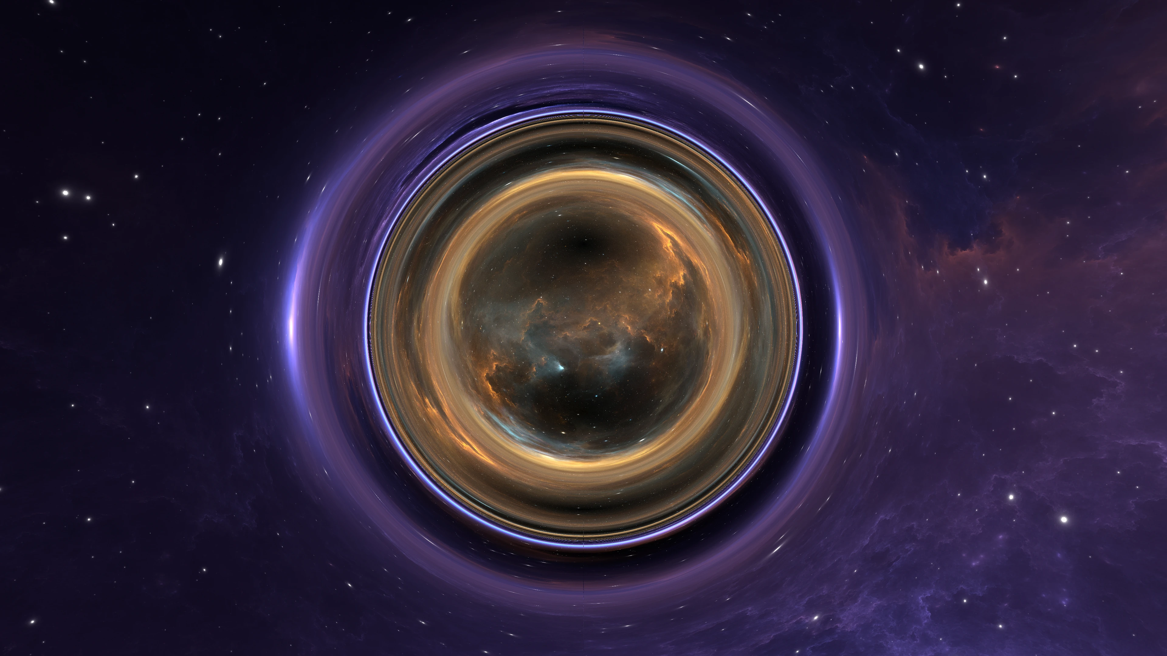
In part 1 we've explored the mathematics behind curved spacetime, and we've derived the geodesic equations that give us the path of light around a wormhole in spherical coordinates:
We are now ready to set up a regular ray tracing scene to render the wormhole. The steps are:
- Position our camera in spacetime, i.e. [begin-latex-inline](t_0, l_0, \theta_0, \phi_0)[end-latex-inline]
- Define our screen by setting a desired field of view, and calculate a unit direction vector for each pixel of the screen, i.e. a vector pointing from the camera position to the pixel
- For a given pixel and its direction vector, calculate the corresponding initial velocity conditions [begin-latex-inline](\dot{t_0}, \dot{l_0}, \dot{\theta_0}, \dot{\phi_0})[end-latex-inline] (they define the direction of the light ray)
- Numerically solve the geodesic equations for [begin-latex-inline](t_0, l_0, \theta_0, \phi_0, \dot{t_0}, \dot{l_0}, \dot{\theta_0}, \dot{\phi_0})[end-latex-inline]
- After tracing the trajectory of the light ray, we map the final [begin-latex-inline](l,\theta,\phi)[end-latex-inline] to a pixel on one of our 2 space images (for this reason, to avoid distortions, the images must be 360 projections). The sign of [begin-latex-inline]l[end-latex-inline] indicates which image to sample from.
We'll use Taichi which allows us to run GPU kernels easily in Python.
Screen
We let the screen be one unit distance away from the camera, and define its size in coordinate units indirectly by defining the field of view [begin-latex-inline]\alpha[end-latex-inline]:
The height of the screen in coordinate distance is calculated with the field of view, and the width is calculated such that the aspect ratio of the virtual screen is the same as the aspect ratio of our actual resulting image in pixels. [begin-latex-inline](W,H)[end-latex-inline] are the width and height of the output image in pixels (the number of squares on the screen in the diagram above).
Direction Vector
For each pixel of that screen we want to compute a unit direction vector that points from the camera to the center of the pixel. However, the camera can be anywhere in the scene. For our implementation, we'll assume we always want to point the camera towards the center of the coordinate system (where the wormhole is). We can find the direction vector by using the spherical coordinates basis vectors. In spherical coordinates we have:
Therefore, the basis vectors are:
Where [begin-latex-inline]\vec{e_l}[end-latex-inline] points radially outwards, [begin-latex-inline]\vec{e_\theta}[end-latex-inline] points downwards from [begin-latex-inline]+z[end-latex-inline] to [begin-latex-inline]-z[end-latex-inline], and [begin-latex-inline]\vec{e_\phi}[end-latex-inline] points to the right from [begin-latex-inline]x^+[end-latex-inline] to [begin-latex-inline]x^-[end-latex-inline]. We can use this basis to find the direction vector for each pixel, however the current unnormalized form is not convenient, so let's normalize:
For every pixel [begin-latex-inline](i,j)[end-latex-inline] of the screen, the direction vector can be computed as:
# orthonormal basis vectors
u_l, u_th, u_ph = # ...

i = # ... pixel row
j = # ... pixel col

# map the center of each (i,j) pixel to [-h/2,h/2] and [-w/2,w/2]
u = (2 * (i + 0.5) / H - 1) * (h / 2)
v = (2 * (j + 0.5) / W - 1) * (w / 2)

# -u_l takes us from the camera to the screen (radially inward)
# u * u_th takes us down some amount of pixels
# v * u_ph takes us right some amount of pixels
d = -u_l + u * u_th + v * u_ph
d /= d.norm()
We basically have the orthonormal basis at the center of the screen, and we want to reach each pixel of the screen: we compute a linear combination of the basis vectors.
4-Velocity
Finally, we need to map the direction unit vector to the velocities [begin-latex-inline](\dot{t_0}, \dot{l_0}, \dot{\theta_0}, \dot{\phi_0})[end-latex-inline]. The velocity vector in the wormhole coordinates is simply:
Since the normalized direction vector is written in the same basis:
We can equate both vectors, component-wise, to find the velocities:
Solving the Geodesics
In part 1 we used Euler's method to solve the system of differential equations. However, in practice, the method requires a very small [begin-latex-inline]dt[end-latex-inline] step size to yield good results which considerably slows down the simulation. Instead, we'll use the 4th Order Runge-Kutta method (aka RK4).
We won't do a derivation of the method here, but provide nonetheless some intuition for those unfamiliar with the method.
Assume we have the derivate of the function of interest, [begin-latex-inline]y[end-latex-inline], expressed as a function of itself and the variable with respect to which we derive, and some initial conditions:
1st Order Runge-Kutta is actually just Euler's method that we've been using so far:
We approximate the function with it's tangent near the initial condition [begin-latex-inline](t_0, y_0)[end-latex-inline].
4th Order Runge-Kutta gets a better tangent estimate by averaging 4 steps of Euler's method (at [begin-latex-inline]y_0, y_{1/2}[end-latex-inline] and [begin-latex-inline]y_1[end-latex-inline]):
In our case, [begin-latex-inline]t[end-latex-inline] is [begin-latex-inline]\lambda[end-latex-inline] (the variable we're integrating against); and [begin-latex-inline]y[end-latex-inline] can be any of [begin-latex-inline]\{t,l,\theta,\phi\}[end-latex-inline]. So our case is more accurately described by [begin-latex-inline]f(\lambda,t,l,\theta,\phi)[end-latex-inline]. For the implementation, we'll encapsulate [begin-latex-inline]\{t,l,\theta,\phi\}[end-latex-inline] in a single state vector.
Since our equations don't depend on the variable we're integrating against, [begin-latex-inline]\lambda[end-latex-inline], we can simplify the implementation by removing [begin-latex-inline]\lambda[end-latex-inline] from [begin-latex-inline]f[end-latex-inline]. We'll call the integration step [begin-latex-inline]h[end-latex-inline] instead of [begin-latex-inline]dt[end-latex-inline] to not confuse it with time, and factorize [begin-latex-inline]h[end-latex-inline] outside the [begin-latex-inline]k_i[end-latex-inline]:
Mapping [begin-latex-inline](l, \theta, \phi)[end-latex-inline] On A Sphere
Finally, we convert the last point of the traced ray to a pixel color. We'll load 2 space images from which we'll sample pixels. We'll normalize [begin-latex-inline]\theta[end-latex-inline] and [begin-latex-inline]\phi[end-latex-inline] and map them to the height [begin-latex-inline](H_i)[end-latex-inline] and width [begin-latex-inline](W_i)[end-latex-inline] of the image to sample from:
To decide which image to sample from, we look at the sign of [begin-latex-inline]l[end-latex-inline], which must be positive in one universe and negative in the other.
Final Code
Here's the final code, you just need to replace the paths to 2 equirectangular projection images (360 panorama). You may find interest in this projection of our Milky Way galaxy from the European Space Agency, or non-space related examples on Wikipedia.
import numpy as np
import taichi as ti

ti.init(arch=ti.gpu, default_fp=ti.f32)

Vector6f32 = ti.types.vector(6, ti.f32)
Vector3f32 = ti.types.vector(3, ti.f32)
Field = ti.template()


@ti.func
def r_of_l(l: float, r0: float) -> float:
    return ti.sqrt(l * l + r0 * r0)


@ti.func
def r_prime_of_l(l: float, r0: float) -> float:
    return l / ti.sqrt(l * l + r0 * r0)


@ti.func
def rhs(state: Vector6f32, r0: float) -> Vector6f32:
    l, th, ph, vl, vth, vph = state[0], state[1], state[2], state[3], state[4], state[5]

    r = r_of_l(l, r0)
    rp = r_prime_of_l(l, r0)
    rpr = rp / r
    st = ti.sin(th)
    ct = ti.cos(th)

    # make sure we don't divide by zero by adding an epsilon
    # also make sure we don't flip the sign by making epsilon signed
    st_safe = ti.select(ti.abs(st) < 1e-12, ti.select(st < 0, st - 1e-12, st + 1e-12), st)

    # geodesic equations in wormhole space
    # at = 0
    al = r * rp * (vth * vth + st * st * vph * vph)
    ath = -2.0 * rpr * vth * vl + st * ct * vph * vph
    aph = -2.0 * rpr * vph * vl - 2 * (ct / st_safe) * vph * vth

    return ti.Vector([vl, vth, vph, al, ath, aph], dt=ti.f32)


@ti.func
def rk4_step(state: Vector6f32, h: float, r0: float) -> Vector6f32:
    k1 = rhs(state, r0)
    k2 = rhs(state + 0.5 * h * k1, r0)
    k3 = rhs(state + 0.5 * h * k2, r0)
    k4 = rhs(state + h * k3, r0)
    return state + h * (k1 + 2.0 * k2 + 2.0 * k3 + k4) / 6.0


@ti.func
def trace_geodesic(state: Vector6f32, h: float, hmax: float, r0: float) -> Vector3f32:
    num_steps = ti.cast(hmax / h, ti.int32)
    for _ in range(num_steps):
        state = rk4_step(state, h, r0)
    # return the last (l, theta, phi) of the trace
    return ti.Vector([state[0], state[1], state[2]], dt=ti.f32)


@ti.kernel
def make_initial_states_kernel(l0: float, th0: float, ph0: float, r0: float, fov: float, height: int, width: int, states: Field):
    ct, st = ti.cos(th0), ti.sin(th0)
    cp, sp = ti.cos(ph0), ti.sin(ph0)

    u_l = ti.Vector([st * cp, st * sp, ct], dt=ti.f32)
    u_th = ti.Vector([ct * cp, ct * sp, -st], dt=ti.f32)
    u_ph = ti.Vector([-sp, cp, 0.0], dt=ti.f32)

    half_h = ti.tan(fov / 2.0)
    half_w = half_h * (width / height)
    r = r_of_l(l0, r0)

    for i, j in states:
        u = (2 * (i + 0.5) / height - 1) * half_h
        v = (2 * (j + 0.5) / width - 1) * half_w

        d = -u_l + u * u_th + v * u_ph
        d /= d.norm()

        # we use the dot product to extract components of d along u_l, u_th, u_ph
        vl0 = d.dot(u_l)
        vth0 = d.dot(u_th) / r
        vph0 = d.dot(u_ph) / (r * st)

        # if you also want to simulate time, you'll need to add t to the RK4
        # intregator and force light-like geodesic by setting:
        # t0 = 0
        # vt0 = ti.sqrt(vl0*vl0 + r*r * (vth0*vth0 + st*st * vph0*vph0)

        states[i, j] = ti.Vector([l0, th0, ph0, vl0, vth0, vph0], dt=ti.f32)


@ti.kernel
def run_simulation_kernel(h: float, hmax: float, r0: float, states: Field, geodesics: Field):
    for i, j in states:
        geodesics[i, j] = trace_geodesic(states[i, j], h, hmax, r0)


@ti.func
def sample_texture(texture: Field, th: float, ph: float) -> float:
    H = ti.static(texture.shape[0])
    W = ti.static(texture.shape[1])
    two_pi = 2.0 * ti.math.pi

    # mod phi as it loops around the globe, so phi=0 <=> phi=2pi
    ph = ti.math.mod(ph, two_pi)
    ph = ph + two_pi if ph < 0 else ph
    # do not mod theta because theta=0 <!=> theta=pi, clamp to ensure normalization works
    th = ti.math.clamp(th, 0.0, ti.math.pi)

    x = (ph / two_pi) * (W - 1.0)
    y = (th / ti.math.pi) * (H - 1.0)

    ix = int(ti.math.clamp(x, 0, W - 1))
    iy = int(ti.math.clamp(y, 0, H - 1))

    return texture[iy, ix]


@ti.kernel
def render_image_kernel(geodesics: Field, output: Field, space1: Field, space2: Field):
    for i, j in output:
        l = geodesics[i, j][0]
        th = geodesics[i, j][1]
        ph = geodesics[i, j][2]

        # sample from a different image based on where the ray ended up
        output[i, j] = ti.select(
            l > 0.0,
            ti.cast(sample_texture(space1, th, ph), ti.f32),
            ti.cast(sample_texture(space2, th, ph), ti.f32)
        )


def load_texture(filename: str) -> Field:
    image = ti.tools.imread(filename, channels=3) / 255.0
    field = ti.Vector.field(3, dtype=ti.f32, shape=image.shape[:2])
    field.from_numpy(image.astype(dtype=np.float32))
    return field


def main():
    width = 1920
    height = 1080
    fov = 80 * ti.math.pi / 180.0
    h = 1e-3
    hmax = 20.0
    r0 = 1.0
    l0 = 5.0
    th0 = ti.math.pi / 2.0
    ph0 = 0.0

    states = ti.Vector.field(6, dtype=ti.f32, shape=(height, width))
    geodesics = ti.Vector.field(3, dtype=ti.f32, shape=(height, width))
    output = ti.Vector.field(3, dtype=ti.f32, shape=(height, width))
    space1 = load_texture("space1.jpg")
    space2 = load_texture("space2.jpg")

    print(f"Generating initial states for {width * height} rays...")
    make_initial_states_kernel(l0, th0, ph0, r0, fov, height, width, states)

    print("Tracing geodesics...")
    run_simulation_kernel(h, hmax, r0, states, geodesics)

    print("Rendering image...")
    render_image_kernel(geodesics, output, space1, space2)

    print("Saving image...")
    ti.tools.imwrite(output.to_numpy().transpose((1, 0, 2)), "wormhole.png")

    print("Done.")


if __name__ == '__main__':
    main()
Travel through a Wormhole
At this point, we can simply move the camera's initial position along a desired path and render multiple images that we combine into a video. This is what I did in this 45 seconds 4K animation: